Finite stress, scaling maps and shell charges · Part 2

per site by 1. This is finite induction over the stops: the initial insertion estimates give the terminal case, and at each earlier stop the chart transport estimate and its forced-source estimate give the next case. The delay conditions put every coupling in this finite induction in the same interval ], so the chosen budgets apply throughout.

For completeness, the final conversion of these density bounds to a rooted Wilson bound can be written explicitly. Let be the number of width-stop sites, which is also the number of reflected chambers. Ifis a fired subset of the markers, the weighted coefficient estimate for the pushed density and the positive partition-function lower bound give

Searchable transcription

∥⟨
Y
chambers
copy Dq⟩Wilson∥RZ|q|
k
≤exp{ZP −4 dim g log g} .
(IG6)

The parameter 0 here is the width-stop small-field parameter, with is its per-site protection bound with source count at most 1 +. The partition estimate applies to the actual positive course density. Its comparison with the reference density uses the two-sided exponent error bounded by: one side bounds the numerator and the other side bounds the positive denominator, so their errors are both included in

Taking the-th root in (IG6) is legitimate because 0. The width-stop allocation was chosen so that 4 dim g log

The rooted chamber seminorm therefore obeys

Searchable transcription

∥Dq∥root ≤eIk
R|q|
k
≤eIk
Rk
= e−Ik = εk.
(IG7)

The middle inequality uses1 and1. The allocation is eventually available because the finite source-count ticket at the width stop is bounded by; this is the delayed station choice, made simultaneously with the finitely many chart, insertion and transport inequalities. Applied to the two singleton modes and the pair mode, (IG7) is the asserted common bound for (IG1). These are bounds for the actual Wilson law, before any character is selected.

Here is why this gives the same bound for the character reading of each corresponding continuum polynomial. Let be any finite linear combination of distinct-point words with the rooted bound , and let be its compressed whole-word operator. For every integer1, place 2 copies of , with alternating reflected conjugation, in chambers separated by a distance parameter sufficiently large volume these are distinct chambers. The finite chessboard inequality bounds the absolute expectation of their product by At fixed, the ordered lattice limit preserves this inequality; the comparison filter lies below that same ordered-limit filter and the coefficient representatives converge there. Then let. The long-word compression limit, expanding the finite linear combinations without commuting their operator factors, gives

Searchable transcription

⟨Ω0, (B∗B)nΩ0⟩≤c2n.

Searchable transcription

The character decomposition therefore gives
Z
|χ(B)|2n dμ(χ) ≤c2n.
(IG2)

It follows that for every character. Indeed, if, continuity provides an open neighborhood of, a number, and a positive measure of that neighborhood, on which

. Full support gives 0. Then (IG2) implies for every, an impossibility as. This includes = 0. The two limits here have their stated order: first the lattice limit at fixed copy count and separation, then separation to infinity, then the integer Let and denote the continuum one-and two-point readings in any one character. Applying this argument to (IG1), and using the unit reading 1, gives

Searchable transcription

|uj −mj| ≤c,
|u01 −m0u1 −m1u0 + m0m1 −z| ≤c.

Searchable transcription

The exact decomposition

Searchable transcription

u01 −(m0m1 + z) = [u01 −m0u1 −m1u0 + m0m1 −z] + m0(u1 −m1) + m1(u0 −m0)

Searchable transcription

proves
|u01 −(m0m1 + z)| ≤[1 + |m0| + |m1|]c.
(IG3)

Thus the Gaussian comparison follows from three specified interacting rooted estimates, not from an assertion that the interacting measure converges to a Gaussian measure.

Searchable transcription

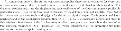
At comparison index i, the station construction supplies these rooted estimates for every pair
of basis labels through degree i, with c = εi →0, uniformly over its fixed position window. The
Gaussian readings mj, z are the singleton and pair coefficients of the Gaussian moment profile. In
particular m0m1 + z is its full two-point coefficient, by the defining cumulant identity. Write Qi(x)
for the rounded position tuple and riQi(x) for the actual physical tuple. If x is generic and has a
neighborhood in the comparison window, then Qi(x) →x, so it is eventually generic and stays in
that window. Smoothness of the free hierarchy implies convergence, and hence boundedness, of its
two singleton readings at Qi(x). Equation (IG3) yields convergence of the interacting two-point
reading to the free two-point reading at x.

The finite-cutoffrepresentatives of a free label converge, along the retained ultrafilter, to a linear lift. Projecting that lift gives the continuum map. The finite station bounds pass to these limits because the lattice moments with converging finite-dimensional coefficient labels have the calibrated ordered limits. The station construction also preserves the unit, conjugation and signed motions. The free detector proves eventual injectivity of; the field-dimension bound gives surjectivity, so these maps are eventually isomorphisms at each fixed degree. Replacing finitely many exceptional initial maps by any fixed isomorphism leaves all limits unchanged.

Searchable transcription

The conclusion also holds for convergent moving free labels vi,0, vi,1. To see this without assum-
ing a uniform norm bound on all interacting bilinear forms, fix a basis ea of the degree-d free space
and expand
X
v a
i,0v b
Bi(vi,0, vi,1) =
i,1Bi(ea, eb).
a,b

Each basis-pair value converges by (IG3), and every displayed coefficient converges. There are finitely many summands. Their limits are therefore exactly the free bilinear form evaluated at the limiting labels. This is the moving-label comparison used for the normalized centered trace.

We finally justify the universal radius selection used in (TLim1). Given an arbitrary positive sequence0, a fixed finite degree horizon, any lower bound on the sequence index and station depth, and any positive radius ceiling, the station construction supplies a later sequence member below that ceiling whose value is exactly the station’s scale radius. Its purchased comparison bounds include the three modes in (IG1), the bounded coefficient lifts and the smeared comparison estimates through that horizon. All their error thresholds can be met together because only finitely many basis pairs and modes occur at this horizon. Recursively increase the horizon to, require a larger sequence index and station depth, and set the next radius ceiling equal to half the radius

Searchable transcription

just chosen. This produces a strictly increasing subsequence map, strictly decreasing chosen radii,
and station depths tending to infinity. At each fixed degree all its comparisons hold eventually.
The exact radius matching has an elementary interval argument. Write Mk ≥1 for the calen-
dar’s magnification monitor and ρk(b) = akMb
k for the station gap. Eventually Mk ≤Mk+1, and
the purchased block bound gives Lk ≤Mk+1. Thus, for b ≥0,

Searchable transcription

ρk(b) = ak+1LkMb
k ≤ak+1Mb+1
k+1 = ρk+1(b + 1).

Also0 for each fixed Given a lower station index, choose beyond these eventual bounds. For 0), take the first with Minimality gives + 1), also when + 1. The continuous function therefore attains. The station family was purchased for this entire interval of exponents; its other charges and interpolation parameters stay fixed over the interval. Consequently this adjustment of preserves its estimates. Given a sequence0, choose a later sequence index below the radius ceiling supplied by this argument, and repeat with a larger. This proves the asserted simultaneous escape of sequence and station indices, with exact equality of radii.

The bounded lifts are then extracted along the already retained ultrafilter and projected as above. Their finite-dimensional limits assemble into one scaling family with exactly those chosen radii. The trace and local-coordinate estimates apply to every such compatible scaling family; they retain the previously fixed physical table and phase. Hence this construction works for the arbitrary sequence supplied to it, including the violating sequence in the proof of the full trace limit.

Source–readout formulation. The comparison never replaces the interacting law by a Gaussian law. Its structure is: (i) a finite identity of densities (the marked density is pushed along the same course, with the same partition function); (ii) rooted bounds (IG7) on three specified corrected modes of the interacting law; (iii) Theorem 23.1, which transfers a rooted bound to every character reading because the phase measure has full support. Step (iii) is a statement about the fibre of phases: a bound valid for the unselected hierarchy descends to each point of the character space, which is stronger than almost-everywhere and is what permits statements about the selected phase. The Gaussian quantities are comparison data of the free sector read on the same labels; the residual of the comparison is and is retained.

Searchable transcription

Theorem 23.1 (From rooted bounds to every character). Let D be a finite combination of distinct-
point words with rooted bound c and compressed whole-word operator B. Then
Z
|χ(B)|2n dμ(χ) ≤c2n
(n ≥1),
hence |χ(B)| ≤c for every character χ.

Consequently, for the continuum one-and two-point readings in any character,

Searchable transcription

|uj −mj| ≤c,
|u01 −(m0m1 + z)| ≤[1 + |m0| + |m1|] c.

Proof. Place 2 copies of with alternating reflected conjugation in chambers at separation; the finite chessboard inequality bounds the expectation of their product by; the ordered lattice limit at fixed preserves it; letting, the long-word compression limit givesΩΩ

and the character decomposition gives the integral bound. If, continuity gives a neighbourhood and with there, of measure 0 by full support, and

fails for large. The order of limits is: lattice limit at fixed copy count and separation, then separation to infinity, then. For (IG3) apply this to (IG1) and use

The exact radius matching at the end of the derivation is geometric: the requested physical radius equals the purchased station radius) for some 1]. It allows the station estimates to be applied at that radius on the same retained physical table and phase. It does not make interacting and Gaussian moments equal at a finite station. Their actual two-point readings satisfy

Searchable transcription

|u01 −(m0m1 + z)| ≤(1 + |m0| + |m1|)c.
(5)

At each fixed degree the purchased errors tend to zero; boundedness of the free singleton readings then gives equality in the specified limit. Prescribed determining-frame normalization elsewhere is an exact finite coordinate calibration, and is distinct from equality of actual hierarchy moments. The universal selection retains this distinction when it is applied to an arbitrary sequence of radii in the full trace-limit argument.

23.3 One calibration matrix for the three panels

The three comparison panels used in (WS1)–(WS17) differ in their point and smear geometry, but have the same finite Taylor order and the same calibration test system. We justify the common matrix, rather than choosing three unrelated solutions. At a fixed degree and sufficiently late stop, the detector matrix of that calibration system is invertible by (PC1)–(PC13). Select the solved chart at one anchor panel. Its defining equations prescribe its pairings with that test system. For any other panel, transport the same local representative and the same Taylor card to its allowed geometry. The support, threshold, and budget equalities make its equations identical to the anchor equations. Uniqueness of their solution then gives the same field matrix at that panel. Signed covariance follows by transporting the solved equations under a signed permutation and again invoking uniqueness. This proves simultaneously the tested-chart and signed-intertwining properties needed in (WS1).

More concretely, the inverse chart is after the field dilation and its engineering-weight factor. Applying the defining calibration equations to a basis proves that it solves those equations; the unit equation gives the unit, and conjugating or turning the equations gives conjugation and signed covariance. Finite dimensionality bounds the finitely many inverse coefficients after the detector lower bound has been paid. These are precisely the coefficients used in the rooted comparison estimate, including on the smear panel. There is no separate choice of an inverse for each spectator word.

For a fixed finite horizon each panel has finitely many local demands, all eventually paid. Take their maximum together with the common detector and monitoring thresholds. At this stage the anchor solution transfers to all three panels at every finer cutoffand every admitted volume. Choose the stops by the cofinal advance already used in (WS16), satisfying these finite maxima and each earlier horizon. Passage to the common coefficient subsequence preserves the tested equations because their finite pairings converge. Therefore the point, displaced-point and smeared comparisons have the same limiting field identification and may be combined in the trace and Ward arguments.

23.4 Common scaling maps and convergence of every derivative

The comparison of a physical field with a free field must use one map for all its readings. Here is the construction, including the compactness and interpolation steps. Fix a finite maximum number of slots, a finite field horizon and a bounded separated configuration window. During this construction these bounds may be enlarged to include detectors and derivatives. The physical table, its null quotient and its limiting correlations remain those already constructed.

Choose radii0 and lattice levels with

Searchable transcription

δk = ank
rk
−→0.
(WS1)

For each free coefficient basis vector at each requested degree, the insertion construction gives a column of physical reference coefficients. Its bound is finite for each fixed, uniformly in the late mesh and large period. These bounds are not asserted uniform in. Extract the finitely many coordinates of each column on their compact balls, first in the mesh limit at a retained period and then in the period limit. Diagonalize over the countable pairs ( The resulting maps initially need not be invertible or commute exactly with the inclusions. Reality, the signed permutation action and the unit pass to the limit since they are finite linear equalities.

The estimates that permit this extraction also supply numbers0, for every fixed word length, with (WS2)

The center and comparison estimates are imposed at levels satisfying

Searchable transcription

am < rk/Q,
6naj < am,
aj < rk/(4Q).

Searchable transcription

The insertion supports are therefore separated before the comparison is taken. On the rescaled
lattice, the aligned comparison tends to the free correlation. On a configuration window in which
all the required coordinate projections have a fixed strict gap, the long finite-difference estimate
gives
|S(Ukv; rkx)| ≤An
k,
|∂xl,αS(Ukv; rkx)| ≤4QAn
k.
(WS3)

Rounding to the rescaled lattice changes a coordinate by); the resulting error vanishes by (WS2). Thus the correlations converge to the free ones on these coordinate-generic windows. All bounds here are for a fixed finite word and fixed window. No uniform bound on all fields or all degrees is being taken.

To fit the coefficient maps, use compactly supported smooth tests in the coordinate-generic part of the separated configuration space. Their readings separate the free quotient. Indeed, a field whose every such reading vanishes has zero correlations there by the fundamental lemma for test functions, and then on the entire separated space by continuity and density. Finite dimension now gives finitely many separating readings at each receiving degree. Spectators in these readings can have larger degree than the field being detected; enlarge the common horizon accordingly. If denotes this finite injective reading map, the physical readings of converge, in matrix norm,

to. Injectivity is open for maps on a finite-dimensional domain: choose a left inverse of when 1, the matrix is invertible. Thus is eventually injective. The previously constructed spanning family gives dimdim , so it is eventually an isomorphism. We make explicit the finite-horizon estimates preceding these readings. A centered budget is the reflection-positive seminorm for every signed or conjugated copy of the one insertion in a reporting chamber. For a word of insertions, take chambers whose centers may be shifted within a finer common chamber. If distinct points have at least one coordinate difference larger than, the

inequalities preceding (WS3) permit these shifts so the inspected insertion cells are disjoint. Apply Cauchy–Schwarz in the positive reflection form successively in the separating coordinate directions. Each insertion contributes its centered seminorm at most; no factor depends on the volume or the microscopic cutoff. Thus the finite Wilson word has magnitude at most Take its ordered mesh and period limits at a coordinate-generic tuple. The fitted coefficients converge in their finite-dimensional balls, and multilinearity permits them to vary along the limit.

The same bound passes to the limiting correlation. On the open set of tuples with some separating coordinate for each pair, the correlation is continuous and the generic tuples have full measure and are dense. Therefore the bound extends to every tuple in that open set. This proves the first part of (WS3) on the entire separated window, including coordinate ties.

For a coordinate-generic tuple with all coordinate gaps larger than 1, move one coordinate a positive rescaled distance. On the microscopic lattice perform the integer displacement in that coordinate. Its physical length tends to. The long finite-difference estimate for the same centered budgets, with available gap), bounds the difference of the two Wilson words by

Searchable transcription

An
k
rkt
rk/(4Q) = 4QAn
kt.
(WS8)

Both endpoint readings converge with their original placements and coefficients. Pass through the ordered limits, divide by, and let0 through endpoints that remain generic. Smoothness identifies the limit with the coordinate derivative and proves the second bound in (WS3). This estimate is uniform on a fixed strict coordinate-gap window. It is not used with tending to infinity near a projection tie.

Searchable transcription

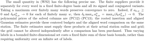
The small quantity in (WS2) has the following precise use.
The finite suppliers provide it
separately for every word in a fixed finite-degree basis and all its signed and conjugated variants.
Taking a maximum over finitely many words preserves convergence to zero.
Indeed, if ak,w ≥
0 and δkan
k,w →0 for each of finitely many w, then δk maxw an
k,w = maxw(δkan
k,w) →0.
The
polynomial prices of the solved columns are (PC12)–(PC13); the rooted insertion and aligned
Gaussian estimates provide these centered budgets and the aligned word comparison on the same
station. The finite estimates must supply these products at their actual station radius and grid;
the grid cannot be altered independently after a comparison has been purchased. Thus varying
labels in a bounded finite-dimensional set costs a fixed finite sum of these basis bounds, rather than
requiring uniformity over an infinite set of labels.

Here is the scale and price bookkeeping in that last statement. For each requested station all degrees through the horizon use one earlier index, with

Searchable transcription

a(k) −→∞,
sk −sa(k) ≤log bβk,
aa(k)
ak
≤bβk.
(WS11)

Searchable transcription

The last inequality follows by exponentiating the preceding one, since ai = e−si. At the comparison
radius rk the actual rescaled mesh is aa(k)/rk = mag−1
a(k). The common finite matrices are taken to
sublimits along the same comparison filter below the retained ordered filter. Each pair of degrees,
each spectator and each placement therefore uses these same matrices and this same radius.
The reverse coefficient transport from a level m to k ≥m has price

Searchable transcription

quotak(v) ≤(am/ak) quotam(v).
(WS12)

Searchable transcription

Indeed one step costs the column allowance Ri+1 ≤Li; multiplying those inequalities gives
Qk−1
i=m Li = am/ak. The solved readout at a(k), followed by its exact field-number and engineering
dilations, consequently supplies a preimage y for every actual coefficient v, with

Searchable transcription

∥y∥≤2a−d
k
quotak(v).

To check the factor two, its approximate matrix differs from the exact awake coefficient by at most half the awake coefficient size, as in (PC7); the triangle inequality bounds the approximate size by twice the awake size. The field shrink is at most one and the comparison magnification at least one, so undoing their positive dilations cannot increase the weighted coefficient size. Formula (WS12)

Searchable transcription

then gives the displayed bound.
This argument applies to the full coefficient space, including
equation directions, before restricting to the physical quotient.
The magnification and each fixed finite sum of its engineering and field-number powers have
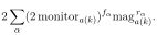
rate zero relative to log bβk. For example the label price is bounded by

Searchable transcription

2
X
α
(2 monitora(k))fαmag rα
a(k).

Searchable transcription

For every ε > 0, each fixed power is eventually at most bβε
a(k) ≤bβε
k; the finite sum has the same rate-
zero property. These are the actual finite-horizon prices used with the rooted insertion estimates.
The centered estimates assert jointly, for a word of length n, the existence of reporting levels m ≤j
such that
am < rk/Q,
n(6aj) < am,
aj < rk/(4Q),
An
k(aa(k)/rk) →0.
(WS13)

The first three conditions give the movable disjoint chambers used in (WS8); the last is exactly the price needed in (WS9). They are imposed together with the aligned moment comparison, not inferred merely from the two-field detector limit. In passing from a basis to bounded arbitrary labels, expand every slot in the fixed finite basis and sum the products of the coordinate norms. The finite sum preserves both the vanishing comparison error and the last limit in (WS13).

Searchable transcription

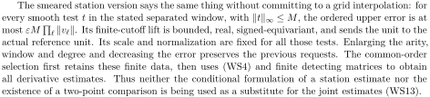
The smeared station version says the same thing without committing to a grid interpolation: for
every smooth test t in the stated separated window, with ∥t∥∞≤M, the ordered upper error is at
most εM Q
l∥vl∥. Its finite-cutofflift is bounded, real, signed-equivariant, and sends the unit to the
actual reference unit. Its scale and normalization are fixed for all those tests. Enlarging the arity,
window and degree and decreasing the error preserves the previous requests. The common-order
selection first retains these finite data, then uses (WS4) and finite detecting matrices to obtain
all derivative estimates. Thus neither the conditional formulation of a station estimate nor the
existence of a two-point comparison is being used as a substitute for the joint estimates (WS13).

The simultaneous centered supplier can be described explicitly; it is stronger than a two-point Gram comparison. Fix a degree cap, an arity cap2, and a compact separated window. The actual construction provides three calibrated panels at exponents, on one family and with the same coefficient matrices. The bounds used for a panel are its solved-column and marked insertion bounds (PC1)–(PC13), together with the rooted comparison of the entire requested finite word. Denote the common monitor by, and write . In the source this is bill( clim thus). A primary comparison radius is), its mesh spacing is ), and a small motion allowance is). Choose the exponents so that

Searchable transcription

c < 0,
b + 6 < a,
e + 5 < a + c,
(a −b)Dn + c < 0,
(a −e)Dn −a −c < 0.
(WS14)

There is no obstruction to these finite numerical choices. Put , and. Then 7 and 0; also all three panel exponents exceed + 6. These are the source’s finite choices. The calibrated panel supplier is chosen with these exponents before extraction.

Here is how that supplier yields centered bounds, rather than merely ordinary moment bounds. For a single basis label, the rooted comparison applied to the singleton at the origin controls the observable minus its free scalar value by the word error0. The centered root seminorm is subadditive, is homogeneous in scalar coefficients, and assigns norm one to the constant observable. Thus its full observable has root seminorm at most 1 +, eventually. Interior support in the centered chamber holds at every translated origin by locality of the observable; translation of the

chamber preserves this root seminorm. This gives a uniform centered bound at the panel’s own width, including its constant part.

Changing the panel magnification from to multiplies a coefficient of engineering degree by. Expand in the fixed finite label basis. The triangle inequality therefore gives the centered price (WS15)

Searchable transcription

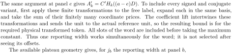
The same argument at panel e gives A′
k = C′Hk((a −e)D). To include every signed and conjugate
variant, first apply these finite transformations to the free label, expand each in the same basis,
and take the sum of their finitely many coordinate prices. The coefficient lift intertwines these
transformations and sends the unit to the actual reference unit, so the resulting bound is for the
required physical transformed token. All slots of the word are included before taking the maximum
constant. Thus one reporting width works simultaneously for the word; it is not selected after
seeing its offsets.
The available plateau geometry gives, for jb the reporting width at panel b,

Searchable transcription

n(6ajb) < ajb−1,
ajb−1
ak
≤Hk(b + 6),
aje
ak
≤Hk(e + 5).
(WS16)

The first follows because one blocking factor tends to infinity. For the other two, the principal plateau length costs); the rounded length and two buffer lengths cost at most five further monitor powers, and passing to the preceding block costs one more. The block factor is bounded by the monitor and its tenth power dominates the fixed covering-size buffers. Multiplying these inequalities gives exactly the exponents + 6 and + 5, rather than changing the comparison radius.

Equations (WS14)–(WS16) now give the simultaneous vanishing products needed in the moving-chamber proof:

Searchable transcription

An
kpk −→0,
(A′
k)nδk/pk −→0,
4nδk ≤pk
eventually.
(WS17)

Searchable transcription

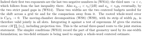
Indeed their first two exponents are the last two negative numbers in (WS14); the third uses −a < c,
which follows from the last inequality there. Also ajb−1 < rk/(2R) and aje < rkpk eventually, by
the two strict panel gaps in (WS14). These two widths are the two centered budgets needed for
the shift across a grid tie and for the comparison away from it.
The rooted whole-word error
is CRεk →0. The moving-chamber decomposition (WS8)–(WS9), with its strip of width pk, is
therefore valid jointly in all slots. Integrating it against a test of supremum M gives the station
error εM Q
i ∥vi∥, including projection ties. This is the actual three-panel route to the joint station
statement. The simpler conditions (WS13) record the part of that geometry used by its one-width
formulation; no two-field estimate is being used to supply a whole-word centered estimate.

Searchable transcription

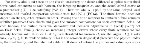
For clarity about existence on the chosen trajectory, the dense calibrated supplies retain fixed
three-panel exponents at each horizon, the foregoing inequalities, and the actual solved charts at
a predecessor g(k) →∞satisfying (WS11). Their availability is paid by the same delayed local
insertion and marked comparison schedule used for (PC1)–(PC13). The finite horizon does not
depend on the requested extraction order. Passing their finite matrices to limits on a fixed common
subfilter preserves those charts and gives the smeared comparisons for their continuum fields. At
each horizon, the finite-dimensional derivative and inclusion adjustments in (WS4)–(WS7) act
on these fields. Finally choose an increasing integer horizon whose every finite requirement has
already become valid at index k: if KD is a threshold for horizon D, use the largest D ≤k with
maxj≤D Kj ≤k. It tends to infinity. This is the common diagonal; it preserves the physical index
k, the fixed family, and the inherited subfilter. It does not retune the grid for individual spectators.