The common continuum hierarchy

The common continuum hierarchy

Two limits with different quantifiers. At each suitable fixed physical period, transported insertions and their two families of bounds establish a full mesh limit. Denoting a tested lattice moment by), the required conclusion has the order

Searchable transcription

rp(t) = lim
N→∞MN,p(t),
lim
k→∞rp(q(k))(t) = S(t).

The first limit uses all sufficiently fine meshes. Only the outer period limit uses a selected refinement of the requested period sequence. Auxiliary compact extractions help construct coefficients; identification with the Cauchy limit prevents them from weakening the first conclusion to a mesh subsequence statement.

Smearing, dense-position extension and derivative compatibility each use the norms and test spaces specified below. They do not follow from pointwise recovery alone. The common field quotient is formed on the same extraction and its calibrated equation image. Kernel stability under the nearby finite projections ensures that an invisible direction does not reappear after an inclusion or derivative. This is the concrete congruence check required for operations on the physical label space.

18.1 Fixed-level integrals from actual transported coefficients

Fix level, period, degree and coefficient. Along the chosen increasing finest cutoffs, the transport construction gives a Cauchy sequence of primary coefficient vectors and a Cauchy sequence of captured interaction coefficients on one common dictionary at level The capture realization equals the same transported insertion’s interaction. Thus coefficient convergence is applied to the actual transported insertion, rather than to an independently chosen representative. Coefficient estimates give uniform boundedness and Cauchy comparison over all configurations for primary entries and forced profiles. Fixed spatial pullback, required conjugation and scalar multiplication preserve these. Finite-dimensional paid coefficient norms are bounded; continuous local terms, measurable masks and convergent sums give measurability. Strip the vacuum scalar from restored density, calling it. Its mode is cold density times the selected coefficient of primary polynomial exponential and background-plus-forced field polynomial. Fixed-level flux comparison and insertion comparison make all factors uniformly Cauchy. Finite polynomial operations and continuous maps on compact bounded ranges preserve this. Probability Haar integrals are Cauchy, as are stripped partition functions with a common positive lower bound. Completeness and that bound give the normalized quotient limit. The vacuum scalar cancels exactly, identifying this quotient with the common-normalization insertion integral. This is the link between the fixed-level coefficient construction and the earlier fine-to-intermediate comparison. The lift retains actual captures, dictionary and stripped factors. Recovery commutes with finite restoration and probability integration, preserving this identification and denominator.

Searchable transcription

Uniform mode convergence under the readout.
At fixed (m, p, d, y) write Tn,A for any
restored mode after stripping the scalar vacuum factor, and Zn ≥δ > 0 for the corresponding
stripped partition function. On the framed source put T Z
n,A = Tn,A ◦π. Surjectivity and normalized
Haar pushforward give

Searchable transcription

∥T Z
n,A −T Z
l,A∥∞= ∥Tn,A −Tl,A∥∞,
an,A =
Z
Tn,A dμ =
Z
T Z
n,A dν.

Searchable transcription

Here π∗ν = μ is the fixed-level probability Haar prior, before multiplication by the restored density.
The actual captured coefficients, forced flags and measurable masks are the same in both integrands.
Thus |an,A −al,A| ≤∥Tn,A −Tl,A∥∞; no continuity of a mask is needed. If |al,A| ≤CA, then

an,A
Zn
−al,A
Zl
 ≤δ−1|an,A −al,A| + CAδ−2|Zn −Zl|.

Both terms tend to zero by the retained uniform coefficient construction. The cancelled vacuum scalar is identical in numerator and denominator at every finite cutoff, so this recovered quotient is the original common-normalization mode integral on this fixed level and period.

18.2 Public hierarchy identifications

The public Hilbert space, word domain, vacuum and fields are the reconstructed ones. These identifications keep the lattice limits, OPE terms and reconstructed fields attached to the same table. Labels are the union of graded table fields; phases and probability measure are the character decomposition. Selected and unselected correlations are that table’s evaluations, and OPE data come from its one reader. Recursive smeared-word evaluation gives the identical word vector, so vacuum moments agree without a limit interchange. Taking its inner product with the vacuum proves equality of the moments. Translation, spectral measure and inverse-affine Poincare test action are the original reconstructed objects. Thus the public covariance and spectral assertions follow by literal substitution once their reconstructed counterparts have been proved. Graded pins are injective; label covering and insertion-token representatives give the two separate surjectivity statements. Nontriviality of the field operators follows from the degree-zero unit: its image is nonzero by injectivity and the unit’s nonvanishing; boundary faithfulness then supplies a Schwartz test with nonzero field operator. Resolved whole words have continuous character evaluations and barycenter equal to the unselected expectation, yielding the public mixture formula. The compression-valued moments and character readings in the reconstruction chapter provide the resolved-word placement and barycenter identities used here. The public holomorphic wave uses pinned labels. Ordered Euclidean times recover the original configuration and heat-root value; joint Schwartz tests and shifts are precisely the reconstructed boundary prescription. Holomorphy, heat-root and boundary existence retain their substantive reconstruction dependencies. Its boundary theorem therefore gives the required vacuum moment. The boundary label-quotient argument in the reconstruction chapter proves faithfulness. The final public projection introduces no second quantum field system.

18.3 One family, table and composed refinement

Choose the Wilson family before observables or volume subsequences. Linear supplier floors and nonlinear component floors form one maximum before block lengths; actual width and chart bills form a later maximum, paid by delay on the same clock. This includes flat delay at = 0, so the actual horizon uses the same flat kernels. The explicit order of the pre-length floors, post-length numerical bills and countable width demands is (CAL12)–(CAL18); their consumption gives the flat delay condition at entrance index zero on the run’s actual horizon, as proved there, and the same fixed family is used below. For requested order, first extract for fixed-level parameter limits, then for the continuum table. Use; increasing sequences preserve earlier convergence and () fixes the final volume order. On that table choose reconstructions for all characters, one equivariant OPE reader and trace test. The preceding construction estimates and the subsequent reconstruction, operator-product and trace arguments establish these services on the retained table. Retain reader coefficients and fields through all truncations, then choose contacts in its same basis. This is the quantifier order used by the public theorem and its detailed extension. Every convergence assertion from the first extraction survives the second, because a strictly increasing natural sequence tends to infinity. The lift retains these actual witnesses and their dependency order. Recovery preserves the common table and composed subsequence, together with whole-word phase, operator and boundary identifications, rather than mixing existence choices.

Recovery of the one public system and its retained refinement. Denote the reconstructed word-domain system by ( Ω Φ), where is its energy–momentum projection-valued measure. Its public readout is the identity on these actual objects. If = Ωand

, the public recursion has the same at every step, and hence the sameΩ Here is the graded pin map. This identifies unbounded fields only on the retained common word domain. The two distinct covering maps remain

Searchable transcription

{insertion tokens} ↠{graded fields} −→L =
[
d
ιd(Fd),

where each is injective and the union covers. Their recovery retains the degree-zero unit and the source’s boundary faithfulness argument. For a whole resolved separated word, the retained character reader and barycenter give

Searchable transcription

Sχ(W) = evχ(W),
S(W) =
Z
Sχ(W) dP(χ).

The reader acts on the resolved whole word prescribed by the source. Its weak character continuity supplies the public continuity statement. The pinned holomorphic wave and joint Schwartz test are the same reconstructed objects, so the public boundary reads its already established boundary value along (. Existence of that boundary value retains its reconstruction dependency.

For completeness, if denotes any quantity whose first extraction converges, recovery on the retained final refinement gives

Searchable transcription

lim
n→∞ag(w(n)) = lim
n→∞ag(n),
f(g(w(n))) = (f ◦(g ◦w))(n).

This is subsequence preservation on the same Wilson family and common table. The source record keeps the pre-length maximum of supplier floors, then the lengths, then the maximum of actual width/chart bills, and then the delay on that clock, including its flat = 0 condition. On the final table it retains the character reconstructions, the single equivariant OPE reader at every truncation, and then contacts in that reader’s basis. Recovery reads this ordered witness record and therefore preserves the shared family, horizon, table, volume order and OPE prescription.

18.4 Full fixed-volume mesh limits and classical derivatives

At fixed intermediate level, Confluence means eventual uniform boundedness and uniform Cauchy comparison in the fixed configuration space. Finite products and sums preserve it, as do continuous maps on common compact ranges. For eventually measurable functions on probability Haar,

Searchable transcription

|
Z
fN −
Z
fM| ≤
Z
|fN −fM| ≤sup
U
|fN(U) −fM(U)|.

Finite polynomial restoration therefore gives Cauchy numerator and stripped partition integrals. The finite polynomial insertion numerator is built from the scalar-normalized density, transported primary insertions and local error insertions by exactly these operations. Retain before division the fixed-level lower bound

exp[Edges dim(Mat()) log(16

Searchable transcription

where v is its positive threshold and K bounds small-field action and activity costs at coupling at
most 2 bβj, independently of finer N ≥j. The trajectory partition identity identifies this with the
normalized denominator. The scalar factor cancels exactly, proving ratio convergence with the es-
tablished nonlinear Confluence inputs; this is the fixed-level ratio convergence used by Rising.latter.
On a compact collision-free set, thicken compactly without collisions. FixedBounds controls
two extra differences of each word. Coordinate-path telescoping bounds its oscillation by physical

distance; applying it to first differences gives a common discrete-gradient Lipschitz constant Subtract the affine function with gradient frozen at the start. Each residual step costs times endpoint distance; telescoping again gives a uniform quadratic Taylor bound. Next-difference limits require no new subsequence. At choose physical 0 small enough for the neighborhood and Taylor error, then put, eventually between and 2. The long difference quotient has Cauchy endpoint limits. Taylor comparison places it within of the unit next difference. Choose for error at most4, then tail quotients within2 to prove next

Searchable transcription

differences Cauchy at x. Local Lipschitz bounds and address error O(aN) give oscillation control;
dense-set extension yields local uniform convergence along the original mesh. Repeat for every
word. For word limit fl and next limits ga,l, passing mesh-address approximations through Taylor
yields
X
(ya −xa)ga,l(x)| ≤B|y −x|2.
|fl(y) −fl(x) −
a

Searchable transcription

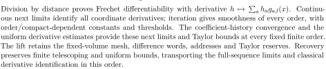
Division by distance proves Frechet differentiability with derivative h 7→P
a haga,l(x). Continu-
ous next limits identify all coordinate derivatives; iteration gives smoothness of every order, with
order/compact-dependent constants and thresholds. The coefficient-history convergence and the
uniform derivative estimates provide these next limits and Taylor bounds at every fixed finite order.
The lift retains the fixed-volume mesh, difference words, addresses and Taylor reserves. Recovery
preserves finite telescoping and uniform bounds, transporting the full-sequence limits and classical
derivative identification in this order.

Recovery before differences and full-mesh differentiation. Let be the framed configuration readout at mesh, and let ∆ be the physical forward difference in a position coordinate, with divisor. The map is independent of insertion positions. For any finite difference word and the same positioned lattice insertion, coefficientwise pullback therefore satisfies

Searchable transcription

∆l,N(IN ◦πN) = (∆l,NIN) ◦πN.

Searchable transcription

The normalized Wilson reader, including all retained corrections, gives the same correlation FN,l
on the two carriers at every finite mesh. It consequently preserves both the uniform fixed-volume
bounds and the physical lattice Taylor inequality
FN,l(Y ) −FN,l(X) −
X
a
(Ya −Xa)FN,a::l(X)
 ≤B|Y −X|2.

Here are physical mesh positions in the retained compact thickening; and the eventual mesh threshold may depend on that compact and word. For the long quotient) at the source’s addressed point, the same reader yields

Searchable transcription

|FN,a::l(XN) −QN(q)| ≤2Bq,

for all sufficiently fine meshes after fixing 0. Hence its pairwise Cauchy estimate is bounded by . Choose first, then the mesh tail. This is the same full mesh sequence. The classical reader then recovers

Searchable transcription

∂afl = ga,l,
Dfl(x)h =
X
a
haga,l(x),

by dividing the retained quadratic remainder by. Thus all finite word limits, their derivative identification, and the small-field partition lower bound remain attached to the same fixed physical volume.

18.5 Stencil independence, interpolation and dense-position extension

Searchable transcription

For fixed backward/forward reaches b, f ≥0, e = b + f > 0, the normalized stencil [F(x + fea) −
F(x−bea)]/(eaN) averages e unit forward differences at x−bea+jea, 0 ≤j < e. Differences commute
with translation averages; iteration expresses any fixed mixed stencil as a finite average of unit words.
All displacements are O(aN), giving the same derivative limit without an extra reach factor. The
right-closed cube interpolant assigns a left-coordinate subset I weight Q
Q
a∈I θa
a/∈I(1 −θa), where
θa is measured from the right endpoint. Nonnegative weights sum to one; vertices lie within O(naN).
Compact cluster convergence bounds the weighted error by the largest vertex error, proving local

Searchable transcription

uniform interpolant convergence even at ties. This assertion does not require or claim that a finite-
mesh interpolant is smooth at its cell boundaries; lattice differences are taken before interpolation.
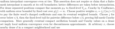
For dense separated positions compare fine moments pN to fixed-level Vj,N, Cauchy by Confluence,
with uniform error bounded by fixed cost over g(j) →∞. Choose positive weights xi = ζi/(|wi|+1)
to pay the finite word’s charged coefficients and sum its eventual weighted bounds. Choose j for
error below ε/4, then the fixed-level tail for pairwise difference below ε/4, proving full-mesh Cauchy
comparison. More generally eventual compact oscillation bounds and Cauchy values on a dense
set imply local uniform convergence even for discontinuous approximants. At arbitrary x, choose
nearby dense d in a compact neighborhood and use

Searchable transcription

|TN(x) −TM(x)| ≤|TN(x) −TN(d)| + |TN(d) −TM(d)| + |TM(d) −TM(x)|.

Completeness gives pointwise limits; oscillation gives continuity. Failure of compact uniform convergence supplies bad points with a convergent subsequence, contradicting oscillation, pointwise convergence and limit continuity. Apply this on fixed-volume periodic collision-free positions, using nonlinear oscillation and schedule-compatible ancestor positions. The previous Taylor arguments then identify all derivative limits. The lift retains reach stencils, cube weights and ancestor positions. Readout preserves finite averages and the same compact oscillation bounds, recovering full-sequence extension without an additional mesh refinement.

Exact stencil, interpolation and dense-position readouts. To distinguish integer addresses from physical positions, write for a mesh address and for its physical point. A fixed-reach stencil has the exact recovery formula

Searchable transcription

b+f−1
X
FN(X + fea) −FN(X −bea)
(b + f)aN
=
1
b + f
j=0
∆a,NFN(X −bea + jea).

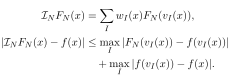
Pullback by commutes with every finite translation and difference in this identity, so mixed stencils retain their exact normalized finite average. If) are the right-closed cell vertices and ) their specified weights, both carriers give the same interpolant and bound

Searchable transcription

INFN(x) =
X
I
wI(x)FN(vI(x)),
|INFN(x) −f(x)| ≤max
I
|FN(vI(x)) −f(vI(x))|
+ max
I
|f(vI(x)) −f(x)|.

Nonnegativity and unit total weight prove this inequality also at cell ties, and both terms vanish uniformly on a compact collision-free set. All lattice differences in this construction precede interpolation.

For the ancestor-position comparison, write for its common finite weighted bill and for the source’s scale function (to separate it from a testing coupling). The same normalized reader gives

Searchable transcription

|pN −pM| ≤2C
G(j) + |Vj,N −Vj,M|.

The weights + 1) and the finite collection of localized errors are retained in. Fixing before the mesh tail preserves the source’s two-level argument. The resulting dense-position Cauchy values and eventual compact oscillation bounds are identical under recovery. Thus the dense-set extension lemma applies to the same full mesh sequence, even when its approximants have discontinuities.

18.6 Smearing and ordered scalar-coupling refinement

Searchable transcription

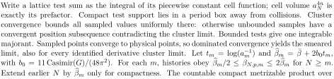
Write a lattice test sum as the integral of its piecewise constant cell function; cell volume a4n
N is
exactly its prefactor. Compact test support lies in a period box away from collisions. Cluster
convergence bounds all sampled values uniformly there: otherwise unbounded samples have a
convergent position subsequence contradicting the cluster limit. Bounded tests give one integrable
majorant. Sampled points converge to physical points, so dominated convergence yields the smeared
m ) and bβm =  ̄β + 2b0tm,
limit, also for every identified derivative cluster limit. Let tm = log(a−1
with b0 = 11 Casimir(G)/(48π2). For each m, histories obey bβm/2 ≤βN,p,m ≤2 bβm for N ≥m.
Extend earlier N by bβm only for compactness. The countable compact metrizable product over

Searchable transcription

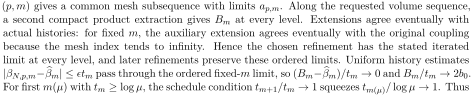
(p, m) gives a common mesh subsequence with limits ap,m. Along the requested volume sequence,
a second compact product extraction gives Bm at every level. Extensions agree eventually with
actual histories: for fixed m, the auxiliary extension agrees eventually with the original coupling
because the mesh index tends to infinity. Hence the chosen refinement has the stated iterated
limit at every level, and later refinements preserve these ordered limits. Uniform history estimates
|βN,p,m−bβm| ≤εtm pass through the ordered fixed-m limit, so (Bm−bβm)/tm →0 and Bm/tm →2b0.
For first m(μ) with tm ≥log μ, the schedule condition tm+1/tm →1 squeezes tm(μ)/ log μ →1. Thus

Searchable transcription

the positive history coupling g(μ) = B−1/2
m(μ) satisfies

Searchable transcription

g(μ)
p
2b0 log μ →1,
g(μ) →0.

Identification with a separately defined position-space diagnostic retains its own comparisontheorem dependency. The lift keeps cell volumes, compact test domains and both refinement maps; recovery preserves dominated smearing and the ordered coupling limits, including this stated scope.

Cell integration and scalar-history recovery. For a compactly supported test on a collision-free-point configuration set, retain the physical cell partition on the lattice test reader is exactly

Searchable transcription

a4n
N
X
X
φ(aNX)FN(aNX) =
Z
φ(sN(x))FN(sN(x)) dx.

Searchable transcription

The support is confined to one fixed compact enlargement in the period box for sufficiently fine
meshes. The source’s compact cluster bound and bounded test give its integrable majorant. Since
the recovered lattice values agree at every sample, both carriers have the same dominated limit
R φ(x)f(x) dx, also for every retained difference-word limit.

Searchable transcription

For the scalar coefficients, the source history record includes all βN,p,m and the auxiliary early
extension. Coordinate evaluation recovers them unchanged, so the retained two compact extractions
give
ap,m = lim
N→∞βN,p,m,
Bm = lim
k→∞ap(k),m,

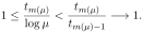
where limits follow the selected mesh and volume refinements respectively. The closed running inequality passes through these two limits at fixed, before. For sufficiently large, the source’s first-crossing index gives

Searchable transcription

1 ≤tm(μ)
log μ <
tm(μ)
tm(μ)−1
−→1.

Together with, this recovers the stated asymptotic history coupling. The readout keeps that history interpretation and the separate comparison dependency for any other coupling diagnostic.

18.7 Common compact extraction and field quotient

Retain two inputs: fixed-period centered root bounds with period-dependent constants, and separately large-period uniform bounds eventually in mesh at each period. For insertions on compact separated positions of margin, choose then with 6. The stencil of each insertion fits its reporting chamber at every sufficiently fine mesh, uniformly in the period: each fixed integer stencil offset times the fine spacing tends to zero, whereas 0 is fixed. Include finite signed/reflected images in root bound. Choose the tiling origin leaving each point at least three reporting widths from boundaries; the inequality leaves a choice in each coordinate. Distinct points occupy distinct chambers. Pull back by prescribed motions/conjugations and apply reflection-positive chessboard to obtain

Searchable transcription

|⟨I1(x1) · · · In(xn)⟩| ≤An.
(CV1)

This argument applies to arbitrary separated tuples; it does not require every coordinate projection of the tuple to be separated. On the generic open set with pairwise distinct coordinate projections, choose compact thickening and projected gap reserve 4. Translation estimates give one-coordinate oscillation at most for Replacing 4 coordinates one at a time stays in the thickening and gives Lipschitz constant 4. Each intermediate tuple is obtained by choosing coordinates from one endpoint or the other, so its distance from either endpoint is at most their distance. Both fixed-period and separate large-period versions hold. Count finite basis words at every degree/arity and compact generic exhaustions. Local countable Arzela–Ascoli gives one mesh subsequence and all fixed-period tables. Pass uniform large-period inequalities to these limits, then take one period subsequence for table. Multilinearity recovers all labels on these same selections. For eventual compact coordinate bounds, replace exceptional early values by a value in each compact set and extract in the countable compact metrizable product. Each coordinate’s original tail agrees, preserving its limit. Additional numerical data are retained by first selecting all active () mesh limits, then using closed large-period compact sets for the outer common subsequence. All active fixed periods remain available. Uniformly bounded idempotent projections have idempotent limits. If injects ker into ker: its kernel would obey. Reverse roles to obtain equal finite kernel dimensions. Detector estimates identify limiting kernels with the exact equation-null space. Transported comparison and step-function smearing make their separated compact-test correlations vanish. The convergence-of-histories chapter establishes the confluence and comparison estimates used in this argument. The lift