14 The analytic stationary graph, loop moments and the cali- brated coupling history · Part 8

are at most the deviation allowance. Regular directions use the anchor-dependent budget (AB1)– (AB4). Forced coefficients use their full configuration domain.

The dependence on the coupling and input activities is continuous in this deviation sense. On a finite set of occurrence addresses, the local integrands and their derivatives vary continuously: the Gaussian covariance and mean, finite Haar factors, cutoffprofiles and stationary coordinates are the actual ones already constructed. Their local integral bounds (ASP2b)–(ASP2c) provide a common integrable majorant. The normalized denominator stays positive in a sufficiently small neighborhood. Differentiation and dominated convergence hence give continuity of each regular derivative supremum on its compact direction and healthy test sets; the full-domain forced bounds use the corresponding full-domain envelopes. For the infinite family, the signed connected expansion gives a common summable majorant on that neighborhood, by (ASP3)–(ASP5). Given 0, first choose a finite address set whose common tail is below4, then use finite continuity to make its sum below2. The two tails contribute at most2. This proves deviation continuity with the actual support weights.

More explicitly, the dependence of the stationary path-only terms on the coupling is affine: if ) denotes one such term, then

Searchable transcription

Aα(β) −Aα(β′) = (β −β′){Aα(1) −Aα(0)}.

The two early envelopes at couplings zero and one give a summable Lipschitz envelope for this difference. The other connected terms are compared by the same marked interpolation before summation. If the input source discrepancy is, their regular and forced absolute envelopes have sums bounded by and for fixed finite, whenever 0. Signed translations cost

Searchable transcription

Z = |Seat(n)| Rim(n) turnFee(B)M.

Reindexing does not change a sum; multiplication by the symmetry normalization and the directionchange allowance gives exactly these factors. Converting a total unweighted envelope to a weighted one costs at most . Thus the outgoing source deviation is bounded by All these constants may depend on this reference torus, budget, fixed path bounds and derivative horizon, but are independent of the approximation depth.

Finally fix a parameter value and an early target 0. Pay2 for its debris tail using (RB8). Choose a parameter neighborhood with full source deviation below); then its restricted debris differences have early allowance at most2. The triangle inequality gives the same tail bound throughout that neighborhood for all sufficiently large depths. A finite subcover of the compact coupling band makes the depth uniform. Applying this to the five fixed reference tori proves the common allowance in (RB7), then (RB4a) and (RB4b), and hence the beacon term in (FCC1). No torus-uniform version of or is used.

Searchable transcription

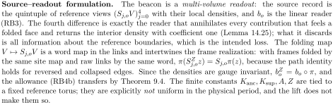
Source–readout formulation.
The beacon is a multi-volume readout: the source record is
the quintuple of reference views (Sj,oV )4
j=0 with their local densities, and bo is the linear reader
(RB3). The fourth difference is exactly the reader that annihilates every contribution that feels a
folded face and returns the interior density with coefficient one (Lemma 14.25); what it discards
is all information about the reference boundaries, which is the intended loss. The folding map
V 7→Sj,oV is a word map in the links and intertwines the frame realization: with frames folded by
the same site map and raw links by the same word, π(SZ
j,oz) = Sj,oπ(z), because the path identity
holds for reversed and collapsed edges. Since the densities are gauge invariant, bZ
o = bo ◦π, and
the allowance (RB4b) transfers by Theorem 9.4. The finite constants Kanc, Ksup, A, Z are tied to
a fixed reference torus; they are explicitly not uniform in the physical period, and the lift does not
make them so.

Lemma 14.25 (Fourth-difference counting identity). Fix a read radius with. A position in a folded coordinate has a type: within of the left face, within of the right face (recording the face and the distance), or interior. For any function of the four-coordinate type,

Searchable transcription

4
X
j=0
ρj
X
x∈torus2(w+j)
f(typej(x)) = f(all-interior type).

Searchable transcription

Proof. A boundary type has a number of preimages under folding independent of j; the interior type
has 2(w−2r+1)+2j preimages. A four-coordinate type therefore has multiplicity a product of four
constant or affine functions of j. The fourth finite difference P
j(1, −4, 6, −4, 1)jg(j) annihilates
polynomials of degree below four, hence every product with a constant factor, and on the product
of four interior factors, whose leading term is 24j4, it equals 4! 24.
Faces and edges of every
codimension are included.

14.18 Derivation and transfer of the reference chart estimate

We first derive the protected-logarithm jet input. Fix the stage and derivative order before the delay. Put, and fineMonitor(). Work at centers with; eventually and the stationary radius exceeds. Every) then satisfies, which is the margin needed for the Gaussian logarithm estimates throughout this ball. Let be the actual protected integral,) its truncated Gaussian approximation with fluctuation cutoff, and = Ωexp(coverLog) 0. The Gaussian comparison on the whole closed ball), using the vertical gap

Searchable transcription

0 ≤I(z) −pV (δ, z) ≤pe−gD2/8,
V (δ, z) ≥a = e−1/2.
(PL1)

The positive omitted tail is bounded by the quadratic Gaussian tail estimate; the local comparison includes the chart and Haar factors. Here Ωis field independent, whereas

is a positive function of the center. The inequalities and the following logarithm argument are pointwise in that center. The cutoffs equal one near zero fluctuation, where the density is strictly positive, so 0. Its Gaussian determinant is positive by the vertical gap. Writing gives 0. Hence the logarithmic discrepancy

Searchable transcription

f = log I −log Ω+ coverLog −log V
satisfies
|f| ≤a−1e−gD2/8,
(PL2)

Searchable transcription

by 0 ≤log(1 + q) ≤q. This is only a value estimate.
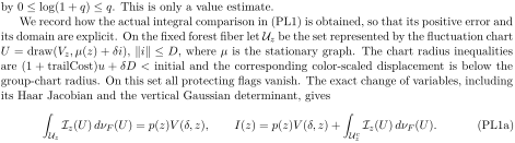
We record how the actual integral comparison in (PL1) is obtained, so that its positive error and
its domain are explicit. On the fixed forest fiber let Uz be the set represented by the fluctuation chart
U = draw(Vz, μ(z) + δi), ∥i∥≤D, where μ is the stationary graph. The chart radius inequalities
are (1 + trailCost)u + δD < initial and the corresponding color-scaled displacement is below the
group-chart radius. On this set all protecting flags vanish. The exact change of variables, including
its Haar Jacobian and the vertical Gaussian determinant, gives
Z
Uz
Iz(U) dνF (U) = p(z)V (δ, z),
I(z) = p(z)V (δ, z) +
Z
Ucz
Iz(U) dνF (U).
(PL1a)

Here is the nonnegative summed fiber density used in the exact push. This is why the comparison has a one-sided error. The outside-field energy bound is paid in the same chart. Denote by the number of free bonds, by 0 the single-bond chart normalization, by the common finite size bound,

and by respectively the local derivative and determinant expenses. With4, its normalized logarithmic expense is

Searchable transcription

YD = −k log wg(β) −RD + vC loopsPrice + K0 + T0.
(PL1b)

Searchable transcription

The fiber complement estimate is
R
Ucz Iz ≤p(z)eYD. It uses the local link reconstruction to put every
small-toll, small-wire configuration in the safety chart. Otherwise its fine or prediction penalty pays
at least the threshold energy. The parameter inequality

Searchable transcription

β meter(vC)u + RD ≤βppenaltym2
0/2

makes that alternative at least as expensive as the fluctuation tail; is a fixed positive safety threshold, not the shrinking radius. The quadratic lower bound within the chart pays the other alternative. Both comparisons use the same actual field and forest fiber. The delay makes2, and also the stronger inequality2. Here the extra expense used to locate a clean chart point is

Searchable transcription

E = β{vCCcl∥z∥5 + vCC′(θ′3 + θ′4)} + K0 + T0 + vCAcoarse/2.

The two terms multiplied by and the loop expense are eventually bounded by one: the field radius has rate16, the threshold has rate2, and the remaining size factors have rate zero. The nondecaying expense is affine in the fine monitor,)fineMonitor(), with bounded by the already fixed polynomial size budgets. The normalization and determinant expenses have the same type of bound. The square4)fineMonitor( dominates this fixed finite list, after the stage parameters and positive are fixed. This proves both inequalities. The stronger one, together with the positive lower bound for the total push, forces a clean point inside; the local chord and displacement estimates then keep all chart flags zero on the surrounding radius- ball. Thus (PL1a) applies throughout that ball. The first inequality and (PL1b) give its error , as claimed. The truncated Gaussian lower bound and its jet estimates use the same size and radius choices. Their derivation is the local Gaussian expansion above; no full-field lower bound for an inverse density is used here.

The Gaussian approximation uses the actual functions constructed above. Keep the retained maximum-norm real coordinates, and give the vertical real coordinate array its Euclidean norm, denoting it by. The linear map) that joins these arrays into the joint maximum-norm array has norm at most one. In this notation set

Searchable transcription

φ(x, h) = F(L(x, h)),
ψ(x, h) = loop(U(x, h)) −
X
e free
log JG(tint(h)e).
(GL0)

Here is the main-action-plus-prediction score (AS1), is its actual fine configuration, loop is the retained quadratic-loop contribution, and is the local Haar density of the chart in the earlier primitive integral. The minus sign makes contain the positive Haar factor. Let) be the vertical Euclidean version of the unique graph (US7), and let) be its Hessian in these vertical coordinates. The equality of counting and Euclidean color squared norms proves

Searchable transcription

Dhφ(x, ρ(x)) = 0,
D2
hφ(x, ρ(x))[z, z] = zTM(x)z,
M(x) ≥(g/2)I.
(GL0a)

Thus the inverse covariance bound used below is; it is the retained half-gap of the actual stationary Hessian.

We explain the common derivative hypotheses for these functions. The joined points used below satisfy

where is the stationary Lipschitz price, enlarged to include the retained identity coordinate. The radius inequalities before (PL1a) put this whole set inside the purchased stationary domain and put every color logarithm inside half the Haar-chart radius. The graph jets are (US8). The score jets follow from (AS6) after the norm-at-most-one map; converting coordinate multilinear bounds to operator bounds costs at most the number of joint coordinates to the derivative order. The loop jets follow by summing the absolutely weighted path jets, multiplied by the fine-site count. A Haar summand is the fixed analytic log composed with a color projection of norm at most 1+dim g, so its order- price is at most its purchased chart price times (2+dim g; summing costs the free-bond count.

The centered determinant jets required below are controlled on this same domain. Differentiate log det) and. Repeating gives a finite sum of traces of products of inverse factors and derivatives of, indexed by ordered derivative partitions. Each trace is bounded by the vertical dimension times the product of the operator norms. The inverse factor has bound 2, and derivatives of are obtained from two score derivatives and the graph chain rule, all at the already purchased higher orders. This gives a finite polynomial price in those jet bounds, the coordinate counts and 2. The value of the centered determinant logarithm follows by integrating its first derivative from zero. These operations give the common price for the graph, classical score, quantum contribution and centered half-log-determinant used below. Its dependence on the auxiliary size bounds is polynomial at fixed derivative order; those sizes have the assigned polynomial logarithmic bounds. Consequently has rate zero. This establishes the hypotheses of the local Gaussian calculation on the entire displaced set, using the actual score, chart and graph.

Define the Taylor-integral expression

Searchable transcription

A(b, x, z) =
Z 1
0
(1 −t)D2
hφ(x, ρ(x) + tbz)[z, z], dt.
(GL1)

Searchable transcription

Stationarity and twice integrating a line derivative give φ(x, ρ(x) + bz) −φ(x, ρ(x)) = b2A(b, x, z),
including b = 0 by the displayed integral. In particular A(0, x, z) = 1
2zTM(x)z. Put

Searchable transcription

G(b, x, z) = 1
2 log det M(x) −1
2 log det M(0) + A(0, 0, z) −A(b, x, z)
+ ψ(x, ρ(x)) −ψ(x, ρ(x) + bz).
(GL2)

Then the same truncated approximation in (PL1) is

Searchable transcription

V (b, x) =
Z
∥z∥≤D
eG(b,x,z)dγM(0)−1(z).
(GL3)

At = 0, multiplying its fixed Gaussian density by the exponential in (GL2) gives exactly the density of. Hence (GL4)

Searchable transcription

This identity retains the moving determinant and covariance; replacing either by its value at zero
would lose the derivative argument.
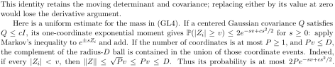
Here is a uniform estimate for the mass in (GL4). If a centered Gaussian covariance Q satisfies
Q ≤cI, its one-coordinate exponential moment gives P(|Zi| ≥v) ≤2e−sv+cs2/2 for s ≥0: apply
Markov’s inequality to e±sZi and add. If the number of coordinates is at most P ≥1, and Pv ≤D,
the complement of the radius-D ball is contained in the union of those coordinate events. Indeed,
if every |Zi| < v, then ∥Z∥≤
√
Pv ≤Pv ≤D. Thus its probability is at most 2Pe−sv+cs2/2.

Searchable transcription

Take P = 1 + Q0(t), where Q0 is the fixed polynomial size budget, and write H = fineMonitor(t).
Eventually P ≤
√
H. For D = dH, choose v = d
√
H and s = v/c. The error is at most

Searchable transcription

2P exp(−d2H/(2c)).
(GL5)

The monitor is chosen to dominate these polynomial size budgets and logarithmic coupling powers, so (GL5) is smaller than for every fixed exponent, after increasing the delay. This estimate is uniform for the moving covariances, since the inverse-Hessian bound gives one common For completeness the derivative price in (GL3) is finite without any derivative of a moving integration set. At order, put

Searchable transcription

Us = 2(1 + C + D),
As = D2Bs(Us, C),
Fs = 2C + 2As + 2Bs(Us, C).

Here bounds the purchased section, score, quantum and centered determinant jets, with two extra score and section orders for (GL1). The affine displacement map in (GL1) has price evaluating its second score derivative on two copies of gives the factor. Integration against , followed by the sum in (GL2), bounds all jets of by. Since) = 0, its first derivative also gives max(). The shrinking chart makes this at most one. Consequently on the fixed cutoffball. Its base Gaussian mass is eventually at least one half by (GL5), so. The exponential composition rule bounds its jets by ); the fixed Gaussian measure is a probability, so integration preserves this bound. The logarithm on the compact interval [] has a finite fixed jet price, giving the joint ()-jet bound). All these prices have rate zero.

Finally (GL2) is unchanged by simultaneously replacing () with (). Symmetry of the cutoffball and base Gaussian makes), and therefore its logarithm is even in . Each of its-derivatives has zero first-derivative at zero. Integrating its second-derivative bounds the difference from its = 0 value by, through order, using the purchased joint order = 0, (GL4)–(GL5) and log) for 11 give an arbitrarily small polynomial value error on the surrounding ball. Apply the interpolation (PL4) below with a rough joint bound and a sufficiently small chosen value exponent. This bounds the-jets of log. Combining the even difference and this zero-parameter estimate gives the asserted Gaussian logarithm jet price at, as well as its lower bound. This proves the Gaussian input used in (PL1) and (RBG2).

The separate rough derivative estimate for the discrepancy on that closed ball is, for a requested order sup (PL3)

For this rough estimate one can avoid estimating an inverse integral on a whole chart. We give the relative derivative bound used in the construction. Write the exact push as an integral over a fixed forest fiber of a finite sum of nonnegative functions

Searchable transcription

I(x) =
Z X
α
aα(U)e−βNα(x,U) dνF (U),
aα(U) ≥0.
(PL3a)

The coefficients include the fine density and all factors independent of the retained coordinate The only-dependence here is the prediction penalty, with the fiber configuration fixed. In particular this argument does not require a nearby point to retain a selected protecting flag. Let

bound the number of coarse bonds. The link product and trace estimates in (AS3) give the penalty jet price colorScale)

The predictor at fixed is a constant group element of matrix norm colorScale; hence this price is uniform in and the finite choice For clarity write the composition polynomial as

Searchable transcription

Bn(a, b) = n!b(2 + a)n.

It bounds the finite partition sum for composition when the inner and outer jets have respective prices at scale one. Subtracting the value of at the center costs a factor two in its jet bound. If bounds the exponential jets at zero, each integrand in (PL3a) therefore has jets through order bounded by its own value times

Searchable transcription

Kn = Bn(2|β|AN, En).

Integrating preserves this relative bound. Differentiation under the integral follows from the same estimate on a neighborhood together with the bounded fine-density envelope and the finite Haar fiber measure. Consequently) for. At each center where (PL1) gives 0, normalize by this single positive value: Its jets at are bounded by, and bounds the logarithm jets at one, the chain rule gives jets of loglog) = log) bounded by). The size of has canceled before estimating. This is the normalization that supplies rough logarithm derivatives uniformly over the surrounding ball.

The other terms of have explicit prices as well. If) is the stationary chart-jet price, set

Searchable transcription

Tn(t) = Bn(2 + 2C(t), C(t)),
On(β, t) = βTn(t) + Tn(t) + C(t).

Composition of the classical action, quantum action and Gaussian determinant on the stationary graph bounds the centered cover logarithm by 2. Let) be the rate-zero Gaussian-log coefficient and put; since1, the Gaussian logarithm jet price is at most Combining the centered logarithms and then restoring the value bound (PL2), which is eventually at most one, gives the rough price

Searchable transcription

M(t) = Bn(Kn(2y, r(t)), Ln) + 2On(2y, t) + 2Q(t) + 1,
n = j + 1.
(PL3b)

The actual coupling lies below 2, so positivity and monotonicity of these polynomials justify that substitution. The bond-count bound), chart coefficient) and) have rate zero. Thus has rate zero, has rate, and) has rate. The cover term has rate one and the Gaussian term rate zero. Their sum has rate at most + 1, and hence is eventually at most. This proves (PL3), including the zeroth derivative by (PL2). It uses actual integral derivatives and the surrounding ball, rather than differentiating the small value error.

Here is the interpolation and its order of choices. If on a ball of radius and , integration along unit directions gives

Searchable transcription

∥Di+1h(0)∥≤2vi/s + Cs.
(PL4)

For multilinear derivatives one tests unit vectors before applying this line estimate. Suppose rough derivatives through order + 1 are bounded by on a ball of radius 0. For any target

exponent, a sufficiently small value bound on that ball implies every jet through order at its center is bounded by. At order zero take. For the step from order to + 1, choose

Searchable transcription

c = a + max(0, d −b) + 1,
b′ = b −1 −c,

then use the order- assertion with target and ball exponent to determine Eventually , so the smaller balls around points within of the center lie in the original ball. The induction gives there. Formula (PL4) gives 2 , whose two exponents are strictly below; their sum is eventually at most. Lower jets already satisfy the stronger bound.

Apply this recursion with. It fixes first; then choose the tail accuracy and delay so that (PL2) is at most. Thus the discrepancy jets are bounded by Gaussian differentiation bounds the separate local Gaussian logarithm jets by , with of rate zero. Keeping that term in leaves the discrepancy in (RBG1). Since

Searchable transcription

max
i≤n ui∥DiY (v)∥≤y−2.
(PL5)

This includes = 0. The critical extension and actual chart composition use the already purchased higher jets and finite composition prices. Those prices are fixed before the tail and reference delays. This supplies the input to the rate calculation below and hence (RB6); the retirement argument then uses the resulting bound with its existing delay order.

We supply the quantitative calculation behind (RB6). Put log, and . All derivative orders and stage parameters in this calculation are fixed before tends to infinity. A function of rate is eventually bounded in absolute value by for each Products add rates, a finite sum has the largest of its rates, and multiplication by any fixed constant preserves a rate. Thus a rate strictly smaller than20 gives the bound in (RB6), with coefficient one, after increasing the delay.

Write the actual reference logarithm, before centering, as

Searchable transcription

g = log Ω+ L0 + Y + βf1 + W.
(RBG1)

Here Ωis the field-independent Gaussian normalization; is the logarithm of the normalized protected local integral after its Gaussian main part is removed; is the remaining Gaussian normalization term; is the difference between the prescribed coarse classical action and the fine classical action evaluated on the stationary graph; and is the difference between the prescribed coarse quantum action and the thermal determinant and Haar contribution on that graph. These are functions on the same real primary-coordinate space. In particular (RBG1) is an equality of the actual densities before any estimate is taken.

For a function, use the scaled derivative bound

Searchable transcription

∥F∥n,A;z = max
0≤q≤n Aq∥DqF(z)∥.

The protected-integral comparison and interpolation (PL1)–(PL5) give, including at the origin. The derivative price of on the radial segment from zero to is

Searchable transcription

d = X(x)gstep(β)2 + ε,
gstep(β) = β−1/2,
(RBG2)

with of rate zero. The integral itself is positive: the Gaussian measure is positive, the protected integrand is nonnegative, and on a nonempty open neighborhood of the zero fluctuation all protecting cutoffs are one and the exponential density is strictly positive. The Gaussian has positive

density there. Its normalizing Gaussian determinant is positive by the vertical Hessian gap. Hence its real logarithm is defined on the chart. The estimates for its derivatives follow by differentiating its absolutely dominated integral and using the logarithm expansion established in (ASP1)–(ASP2). Let1 bound the reference coordinate and site counts, let be the stationary-response price, and let be the sum of the purchased bare-action jet price and the stationary-composition price. More explicitly, the coordinate conversion multiplies an order- multilinear price by the latter composition price is the fixed polynomial clump appearing in the ordered-partition derivative bound. Thus has rate zero. Classical matching removes the jets through order four, giving (RBG3)

The higher jets of, of orders three through, have a price of rate zero. This price is the bare jet bound multiplied by+Λ), together with the same stationary-composition polynomial and. Here is the bounded kinetic correction and Λ is the path allowance. The finite-period thermal comparison bounds its second jet at zero by

Searchable transcription

∥D2W(0)∥≤A0,
A0 = M2{M4m(g)M} Θp e−γc.
(RBG4)

In this formulag) = (1 + dim g) is the fixed color-coordinate conversion factor. The reference side is Θ 0 are the purchased decay constants, and0 is bounded by the adjacent loop allowance. Only the displayed exponential dependence on is used below.

The first jet is smaller than a generic extensive-action bound would suggest. The signed symmetries give(0) = 0, while classical matching gives(0) = 0. Differentiating (RBG1) therefore yields (RBG5)

Taylor’s formula along segments in the chart, with these first and second jets and the third-and-higher jet prices, gives

Searchable transcription

∥W −W(0)∥n,A;z ≤CnA3 + 3{(ε + d)A + A0A2}.
(RBG6)

For orders zero, one and two this follows by integrating the next derivative and using (RBG4)– (RBG5). For an order3, multiply the unscaled bound by. Taking the maximum and enlarging the three low-order contributions gives the factor three. Centering costs at most ; centering costs. Equations (RBG1), (RBG3), and (RBG6) now give

Searchable transcription

∥g −g(0)∥n,A;z ≤dA + 2ε + βKnA5 + CnA3 + 3{(ε + d)A + A0A2}.
(RBG7)

Here. Consequently has rate1. The lower bound on the reference side makes Θ, and hence, have rate1. All remaining prices have rate zero. The respective rates on the right of (RBG7) are at most

Searchable transcription

−23/16,
−2,
−19/16,
−21/16,
−23/16,
−15/8.

Every one is strictly below32, and20. The defining rate inequalities, with a sufficiently small positive slack and then a common delay, therefore make the whole finite sum at most. This derives the quantitative gain rather than assuming that a small integral automatically has a small logarithmic jet.

It remains to explain why the estimate applies to the five reference tori, whose sides need not be physical periods. Choose a physical coarse side divisible by the given reference side; the divisibility requirement was included in the block calendar. Copy the reference forest periodically to this larger