Local nonlinear geometry and Haar realization

Local nonlinear geometry and Haar realization

From a linear predictor to an actual group-valued operation. Quadratic estimates alone do not define a nonlinear block map. This stage constructs logarithmic charts, local minima and group-valued predictors, and compares their derivatives with the flat cochain operators. The raw record retains the chosen chart, branch, guide tree, support, thresholds and all failed-chart flags. A minimum selected on an allowed branch is a conditional operation; it is not a globally unique logarithm of every configuration.

For a physical predictor, an arbitrary coarse frame gives the realized coarse link . Its coarse readout is exactly)). Differentiating this formula includes the frame response and preserves the physical derivative, as in (RF8). The estimates below control this actual operation on its specified domains. They also retain literal healthy masks: an indicator’s boundary is not differentiated as though it were a smooth cutoff. Locality includes the links that determine the flags. The energy, packet and connected-cover estimates subsequently pay for those supports and for the off-chart terms. Discarding a branch, a flag or a path before its estimate is obtained would change the operation being recovered.

Work in the closed matrix image of the compact gauge group. Its real Lie algebra consists of the matrices for which exp() belongs to that image for every real. Let be the orthogonal complement of this real Lie algebra in the ambient real matrix space. If nonzero0, exp and, takefor0. Then and exp() = (exp exp( by closedness; inversion covers negative. Thus is in the Lie algebra. Consequently small with exp must be zero: otherwise normalized directions have a unit subsequential limit in both and the algebra.

Searchable transcription

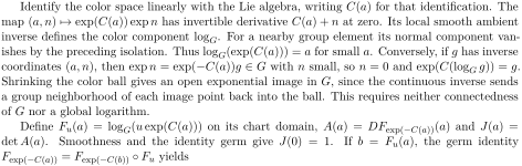
Identify the color space linearly with the Lie algebra, writing C(a) for that identification. The
map (a, n) 7→exp(C(a)) exp n has invertible derivative C(a) + n at zero. Its local smooth ambient
inverse defines the color component logG. For a nearby group element its normal component van-
ishes by the preceding isolation. Thus logG(exp(C(a))) = a for small a. Conversely, if g has inverse
coordinates (a, n), then exp n = exp(−C(a))g ∈G with n small, so n = 0 and exp(C(logG g)) = g.
Shrinking the color ball gives an open exponential image in G, since the continuous inverse sends
a group neighborhood of each image point back into the ball. This requires neither connectedness
of G nor a global logarithm.
Define Fu(a) = logG(u exp(C(a))) on its chart domain, A(a) = DFexp(−C(a))(a) and J(a) =
det A(a).
Smoothness and the identity germ give J(0) = 1.
If b = Fu(a), the germ identity
Fexp(−C(a)) = Fexp(−C(b)) ◦Fu yields

Searchable transcription

J(b) det DFu(a) = J(a).

Shrink the ball 2 and put = exp). The pushforward = (exp is finite and nonzero. On the overlap is injective and its image is the relevant piece of Positivity of turns the overlap law into det Change of variables therefore gives) for measurable Average over normalized Haar measure. Tonelli and right invariance make the left integral). For fixed, the set of for which has measure) by inversion and right translation, so the right integral is). Hence

The set is nonempty and open, and is bounded above and below on the finite-radius ball. Thus both constants are positive and finite, so 0 gives

Searchable transcription

(expG)∗(1ScJ(a) da) = μG|U.

Intersecting arbitrary test sets with proves the full local measure identity. The realized frame construction uses this same, chart, density and normalization; endpoint conjugations preserve the color metric, but no new globally defined chart is introduced by the readout. Product-chart and fluctuation changes below retain their separate Jacobian factors.

12.1 Primitive Haar charts and fluctuation normalization

Searchable transcription

Right Haar invariance sends 1BρcJ(a) da under a 7→expG(a)V to Haar restricted to expG(Bρ)V .
The finite product on active links has density Q
i cJ(ai), with inactive links fixed. The tree-gauge
splitting into active and exterior link coordinates is measure preserving.
Fubini permits active
integration first, then exterior integration, after insertion of the bounded local ingredients. The
powers of c and the Jacobian logarithms come from this product density. Regrouping then produces
the quadratic Gaussian density and the explicit vertex factors; the grafted-signal and Gaussian-
exponent constructions supply the selector implication and that decomposition. Sector selectors

ensure no nonzero contribution is omitted: if , shell access gives chord(, while on the wider shell chord( the logarithm satisfieslog chord() and is inverse to the exponential. The active chart is sufficient because the sector selectors force every active link of a nonzero integrand to lie in that chart relative to its replica background. Choose and . Then = exp with. Outside the chart the cutoffmakes the transformed integrand vanish, so no exterior logarithm value is used in the change of variables. The inserted cutofffunctions can be handled at all color arguments.

The inner-share cutoff lies between zero and one, equals one on and vanishes outside . Thus = 1 on its support. Set) log on the active cutoffsupport. Since(0) = 1 and is smooth positive, loglocally; when 4 is in this radius, globally, including the zero-cutoffbranch. No exterior logarithm is used where the integrand vanishes. For active real coordinates and coupling scale 0, the affine dilation has determinant. Here active coordinates are indexed by active-link/color pairs. Finite-dimensional

change of variables pushes to active-chart Lebesgue measure. Reindexing these pairs into a color vector at each active link is a coordinate permutation and regrouping, preserving measure first on measurable rectangles and hence on all measurable sets. The active part of the original fluctuation is precisely). The dormant matrix is zero on active and identity on vacant coordinates; its energy is2, so for vacant dimension its density is

Searchable transcription

2π)−dve−∥y∥2/2,
Z
C(y) dy = 1,
C(y) = (
√

Searchable transcription

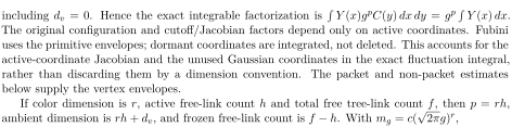
including dv = 0. Hence the exact integrable factorization is
R Y (x)gpC(y) dx dy = gp R Y (x) dx.
The original configuration and cutoff/Jacobian factors depend only on active coordinates. Fubini
uses the primitive envelopes; dormant coordinates are integrated, not deleted. This accounts for the
active-coordinate Jacobian and the unused Gaussian coordinates in the exact fluctuation integral,
rather than discarding them by a dimension convention. The packet and non-packet estimates
below supply the vertex envelopes.
If color dimension is r, active free-link count h and total free tree-link count f, then p = rh,
ambient dimension is rh + dv, and frozen free-link count is f −h. With mg = c(
√
2πg)r,

Searchable transcription

(
√
2π)−dvgrhch = (
√
2π)−(rh+dv)mf
ge−(f−h) log mg.

Searchable transcription

The counts come from the actual finite partition of free links into active and frozen sets. Cancel
mf−h
g
and substitute mg = c(
√
2πg)r to prove the identity. The separate blank-form determinant

Searchable transcription

factor is
e−log det Qblank/2.

A positive covariance in dimension has density

Searchable transcription

(
√
2π)−d exp[−log det Q/2 −z⊤Q−1z/2].

Determinant factors are not dimension conventions. Thus all determinant and Gaussian-volume factors are explicit before the remainder vertices are estimated. Finally retain the raw action split cutΛreducedActionadditiveActivity. The correction uses the whole gap cutcoarseCrown( ) and cancels the retained crown already transferred to the raw density exactly:

Searchable transcription

e−β coarseCrowneβ cutRe−β(cutR −coarseCrown) = 1.

The sector sum is thus the tagged block kernel times the original marked density pointwise. The activity’s summable envelope and bounded sector factors justify integration/summation. The source lift preserves these actual factors under measure readout, including every determinant and sector tag. This is the initial action cancellation in the primitive Mark formula; the marked-integration chapter supplies the local vertex decomposition and primitive-integral estimates completing that formula.

Recovery of the active chart measure. Fix the physical replica background and an active-link set. For each fixed frame the raw active-chart parametrization is

Searchable transcription

Ae = rx expG(ae)Ver−1
y ,
e : x →y,
π(r, A)e = expG(ae)Ve.

Searchable transcription

Left and right Haar invariance followed by the original chart identity therefore gives the same active
density Q
e∈Ea cJ(ae) dae for every r. Integration over normalized frame Haar measure contributes
one. For every integrable test supported in this product chart,
Z
F(π(r, A)) dν(r)
Y
e∈Ea
dν(Ae) =
Z
F((expG(ae)Ve)e)
Y
e∈Ea
cJ(ae) dae,

Searchable transcription

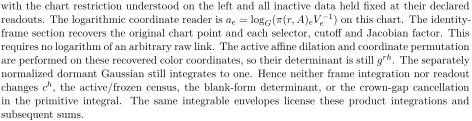
with the chart restriction understood on the left and all inactive data held fixed at their declared
readouts. The logarithmic coordinate reader is ae = logG(π(r, A)eV −1
e
) on this chart. The identity-
frame section recovers the original chart point and each selector, cutoffand Jacobian factor. This
requires no logarithm of an arbitrary raw link. The active affine dilation and coordinate permutation
are performed on these recovered color coordinates, so their determinant is still grh. The separately
normalized dormant Gaussian still integrates to one. Hence neither frame integration nor readout
changes ch, the active/frozen census, the blank-form determinant, or the crown-gap cancellation
in the primitive integral. The same integrable envelopes license these product integrations and
subsequent sums.

12.2 The reference quadratic floor before localization

Let be the active link direction, the physical stacked motion and the orthogonal dormantcoordinate projection. The reference precision is, with

Searchable transcription

u⊤F ⊤Fu = σ2 X
|Du|2.

Searchable transcription

The local geometric estimate is |Lui| ≤ZRi(u) + MCi(u), where Ri is the square root of the sum
of squared physical motions within fixed native radius d, and Ci is the square root of the sum
of squared active link directions within radius 3B. Both use actual torus max-distance and the
actual link census. Set W = P |Lui|2, V = P |Du|2 and Nr = (2r + 1)4L4
block|Axis|. Squaring and
charging occurrences gives
W ≤2Z2NdV + 2M2N3BW.

At the chosen block/stage is fixed and has reference-coupling order2 with the stated width factors. Polynomial width growth permits the eventual condition 22. Absorbing gives for a positive enlarged. Orthogonal active/dormant splitting then proves

Searchable transcription

∥u∥2 = ∥Lu∥2 + u⊤Pdu,
u⊤Pdu ≥0,
u⊤Qu ≥min(σ2/a, 1)∥u∥2.

This derives the floor from physical motion, conditional on the source’s local driving/flattening estimates NF1–NF4, before choosing any covariance; it is not an assumed lower bound for the full matrix. The reference precision is a Gram matrix with an identity completion on dormant coordinates.

Each dormant row and column of the plate is identity and its linear source is zero, including in principal restrictions. The inverse equation therefore gives identity dormant rows and columns in each restricted inverse. Padding a column retains this property because its diagonal lies in its footprint and other entries outside are zero. Symmetrizing the padded inverse gives identity dormant covariance rows/columns, and the mean vanishes there. These exact facts justify the dormant Gaussian used above. Positivity and an upper bound for the whole padded covariance still use the localized inverse-window estimates. Under the source lift the floor is on this actual physical/dormant coordinate space and its isometric section, not on an enlarged space containing extra frame-vertical null vectors.

12.3 Localized inverses and positive finite-window covariance

Searchable transcription

Let A = A⊤≥rI, r > 0, be indexed by coordinates at sites ai, and have width-η (η ≥0) absolute
row and column prices at most X > 0. Principal restrictions inherit the floor by zero extension and
the prices by restricting nonnegative sums. For 0 ≤θ ≤1, θX ≤r/2, take u ≥0, so Au = A + uI
has an actual two-sided inverse. Fix j and conjugate Au by si = eθη dist(ai,aj). If y = A−1
u ej and
wi = siyi, then
(Au + E)w = ej,
Eik = (Au)ik(si/sk −1).

Searchable transcription

Distance and convexity give |si/sk −1| ≤θeη dist(ai,ak). Indeed the log ratio lies between ±θD
and eθD −1 ≤θ(eD −1); for a negative logarithmic ratio v, use 1 −ev ≤e−v −1. The added
diagonal contributes zero to E.
Its row/column prices are at most r/2, so 2|vivk| ≤v2
i + v2
k
gives |v⊤Ev| ≤(r/2)∥v∥2. Pairing the equation with w yields (r/2 + u)∥w∥2 ≤wj ≤∥w∥, with
c = min(1, r/2) this implies c(1+u)∥w∥2 ≤wj ≤∥w∥. The zero-vector case is immediate; otherwise
∥w∥≤[c(1 + u)]−1. Hence

Searchable transcription

eθη dist(ai,aj)|(A + uI)−1
ij | ≤[min(1, r/2)(1 + u)]−1.

This is dimension-uniform and applies to each principal restriction. Take = min(1 and 0 on the positive-width application domain. With at most coordinate labels per site, summing the remaining tail gives a period-independent price at width 2. Indeed the sum of over torus sites is bounded by the corresponding absolutely convergent lattice sum, independently of the period. The full inverse and

Searchable transcription

zero-padded principal inverse columns obey this price. Choose each endpoint-defined window Wj
to contain the radius-B coordinates and lie within radius B+2, and set Kij = (A|Wj)−1
ij inside, zero
outside. Product prices at width 2k bound E = AK −I by XP + 1. The exact principal equation
makes this error zero when i ∈Wj, in particular within radius B. On all remaining entries the loss
of width k supplies e−kB. Its width-k price is therefore at most

Searchable transcription

εB = e−kB(XP + 1).

Searchable transcription

The exact identity K −A−1 = A−1E bounds its error price by PεB.
For C = (K + K⊤)/2, symmetry gives error price price(C −A−1) ≤PεB and price(C) ≤
P. Schur bounds convert the error to a quadratic bound: for a matrix E whose absolute row
and column sums are at most r/2, expanding the double sum and using 2|vivk| ≤v2
i + v2
k gives
|v⊤Ev| ≤(r/2)∥v∥2. Since A ≤XI, A−1 ≥X−1I; this also follows by expanding the nonnegative
form of w −X−1v with w = A−1v. Thus PεB ≤1/(2X) yields

Searchable transcription

(2X)−1I ≤C ≤PI.

The covariance vanishes beyond + 2, and) has width- price at most . All choices are uniform in volume. For the physical plate its prior floor, stencil prices and coordinate census provide; increasing at fixed block/stage pays the error. The physical operator bounds and local driving estimate of this chapter establish these inputs for the plate. The lift transports whole-color-block windows and the original endpoint rule, retaining separately from for the mean. It does not identify a padded principal inverse with the full inverse or assert positive exponential width from an input width of zero.

Recovery of the window covariance and mean. Retain the endpoint-defined windows, their principal inverses and the padded matrix separately from2. For a physical linear source the retained mean is, then for every physical comparison vector

Indeed since, and substitution cancels in the displayed order. Symmetrization of the covariance therefore does not authorize replacing this mean by. For a section and readout with, realize the physical Gaussian by the pushforward Its ambient mean and covariance are and, and its readout is exactly. In particular

Searchable transcription

p(jμ) = μ,
p(jCj∗)p∗= C.

These are covariance pushforward identities, distinct from the pullback of a precision form. The realized Gaussian is supported on the declared section. No ambient Lebesgue density or inverse in frame-vertical directions is introduced. Pulling test functions back by and restricting through recovers the original Gaussian integrals and their dormant factors. Window error, finite range, positive floor and upper bounds are read in the original physical coordinates and transported section norm, with the same site census and widths. Thus the finite-window approximation remains the original one, and both its residual and its mean recover exactly.

12.4 Axial gauge and bounded local logarithms

For finite cover support, let sum internal positive-link chords and sum wholly internal plaquette chords, with boundary/incomplete terms zero. Both are nonnegative and is gauge

invariant. An ordered list of distinct axes defines a slab with those coordinates in [] and the others pinned. From a root in the slab, travel first in the first listed axis to the corresponding coordinate of, then in the next axis, and so on. The remaining coordinates are pinned, so this route ends at; its ordered link product is). Extending the list by axis makes every internal -link identity in this gauge, since the routes to its endpoints differ by precisely that final link.

With those links identity, the plaquette and chord triangle inequalities give

Searchable transcription

| chord U(x + ej, i) −chord U(x, i)| ≤chord hol(□(i, j), x).

Apply the chord triangle inequality to and its inverse for the two horizontal links. Reversing the axis order only inverts the holonomy and preserves its chord. Summing the four positive axes over a slice bounds the change by four times the adjacent-layer plaquette sum; telescoping within the slab gives. All layers used by the telescoping sum lie inside the slab; adding the unused nonnegative layers proves this bound even when the two slices are far apart. Inductively a root exists with for listed axes. The base is a single site. Choose a minimum-face-sum slice for the next axis, whose face sum is at most + 1), since the slice face sets are disjoint subsets of the full slab face set. Apply the prior root construction there, and extend its routes. The chosen slice edge sum is unchanged. The new links are identity and the slice comparison gives the claimed next bound after summing slices. No small-curvature assumption enters root existence.

For four axes this gives 16(2. A periodic radius- patch with plaquette chords at most hasPlaqAxes. Lift the patch to that box and apply the preceding construction. When 2 its box lift is injective; the route gauge descends and extends arbitrarily elsewhere. If, each radius- bond lies within the box, and

Searchable transcription

chord((z · U)(b)) ≤16(2r + 1)5|PlaqAxes|q.

The lift carries the same patch and gauge, including its nonwrapping condition; abstract frame freedom does not enlarge this geometric domain.

The local analytic logarithm has log 1 = 0, givinglogon a small matrix ball. Shrink the ball for the local exponential inverse. Sincemat(= colorScale chord(), this yields constants 0 with exp(log andlog chord() for chord at most. Set the field to this logarithm on the specified interior patch and zero outside. If its chords are at most , the global field is bounded by and recovers the patch links; boundary continuity is not required for this finite lattice field.

For an analytic map, its series identifies the directional derivative with the bounded derivative The first two terms and uniform remainder on one fixed ball give and Applied to the exponential they bound its chord linearly. For the four-factor plaquette curvature the derivative is, yielding an actualcurvature versus discrete-curl error uniformly in position and volume, including repeated edges, because each of the four arguments is bounded by the same field norm. Finally expanding 1) and using unitary invariance of the Frobenius norm together withcolorMat(= colorScalegives

Searchable transcription

∥Ad(U)a −a∥≤2 colorScale chord(U)∥a∥.

Induction along a walk gives chord of its transport at most its length times, with inverse-link chords unchanged. These are the nonlinear/local bounds transported through the actual realized chart and route data.

12.5 Quantitative nonlinear and flat row comparison

Set widen(; cutoffs read actual path length, including winding. A path slot reads a plaquette after adjoint transport along its walk from the reading site. In a chart field , link chords are at most, curl at most and curvature-minus-curl at most A retained transport slot of length at most changes its curl by at most 2 colorScale Hence slot-minus-curl is bounded by widen,(1 + 2 colorScale). For an omitted slot of lengthwith and stage width

Searchable transcription

1 ≤eσle−σR/d ≤eσlwiden(R, h, σ/d).

Searchable transcription

With P
i |ui|eσli ≤paths, the omitted-slot inequality pays its whole linear curl, and absolute
summation of retained errors and omitted linear terms gives

plotted(exp widen(

Searchable transcription

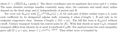
where C =
√
directAch+paths J. The direct coordinate uses its quadratic face error and h ≤widen.
The same absolute envelope handles countably many slots; the constants and small chart radius
depend on the fixed stage and d, independently of period and R.
For cover row Kab(u) with P
u eη|u||Kab(u)| ≤A, for each pair of finite residue types a, b, route
each coefficient by its designated adjoint walk, retaining it when d length ≤R and only in its
endpoint congruence class. Assume d length ≤D(1 + |u|). The full flat term is Kab(u)I without
cutoff. Unitary transport bounds the routed norm by |K|. With link chords at most Cchh, retained
transport differs from identity by at most 2 colorScale CchRh. For omitted terms the route inequality
gives ηR/D ≤η + η|u|, hence 1 ≤eηeη|u|e−ηR/D. Thus either error is bounded by

Searchable transcription

J widen(R, h, η/D)eη|u||Kab(u)|,
J = 1 + 2 colorScale Cch + eη.

Each cover displacement belongs to exactly one endpoint congruence class, even for many windings. Summing absolute majorants first on the cover costs only the finite residue census. Absolute convergence permits interchange of these nonnegative bounds, even on short tori with many windings. For types, bounds row and column sums of both matrices and gives difference price widen.

Same-level coordinate routes have length; residue-to- routes have length at most . Both admit. Replica links are identity or original coarse links and preserve the chord bound. For the rows take = max(max(0) and), then maximize their costs with one and intersect chart radii. Constants are chosen after the fixed uniformly in period/cutoff. At arbitrary realized frames the flat identity-color row becomes its endpoint-conjugated row; readout transports the same comparison, rather than comparing to an untransformed identity in unrelated frame coordinates.

12.6 Clean-hull guides and signed stationary cancellation

The guide is the pair of coarse response fields, compared with flat applied to The flat row vanishes on that field by flatN = 0, because, including harmonic coordinates. On a clean radius-4 hull agreeing with exp, room inequalities contain the row reach = till() and the plotted field’s further +4 sites. Cleanliness makes the retained indicator and clipping factor min(1 temp toll) equal to one there, and locality replaces the row by its value at exp

If the nonlinear row has price, its difference from flat row price, and the plotted/linear field discrepancy is at most with linear field bound, write(exp = plotted(exp and). The exact decomposition is

Searchable transcription

Bf −Dg = B(f −g) + (B −D)g,
∥Bf −Dg∥≤XU + XWZ.

These substitutions hold only on that same hull. The kernel-chart and plotted-chart estimates supply positive constants. Here is the lower-stage width divided by the positive block length. The source choices are) widen(till() and

Searchable transcription

e(x) = XU(x) + X widen(till(x), H(x), s)M(x).

With eventual nonnegative rate- and the actual radius/cutoffbounds, widening retains that rate because it is a radius factor times plus an exponentially small cutoffterm. The products in therefore have rate1. It bounds both guide discrepancies and nonlinear, whose linear part is zero.

Choose together the supplied quadratic beds, their attached path realizations, positive floors, diagonal/roll identities and invariance under signed coordinate changes. Let be their installed stationary map and its extracted fine-field matrix for the chosen forest. Then letprobe The diagonal identity is + penalty

Pairing each color coordinate proves fine shifted energy plus penalty residual norm squared equals coarse energy, including harmonic modes. Signed covariance of the actual nonlinear predictor and noise energy, applied to exponentiated and divided by, transfers this identity to every signed orientation. Bed invariance supplies the other terms; entrywise isotropy is not assumed. Let be the transformed coarse, shifted fine and noise linear moment fields. The attached path realizations and floors identify moment-square sums with bed energies; all norms here are finite counting sums of squared color norms. Thus . Set Since = 0, the roll identities give in the finite counting inner products. Pairing with gives and. Expanding therefore yields

Nonnegative summands prove equality row by row, hence linearCost equals linearGuide in every signed orientation. Subtraction gives the uncut spring cancellation. The source lift preserves the same beds, forest, signed action and counting metric, so this cancellation is recovered without replacing a nonlinear cutoffidentity by a global assertion outside its clean hull.

12.7 Nearest group points and analytic focus

Use the real Frobenius inner product. Compactness of the closed unitary matrix group gives a nearest group point to every matrix, and left/right group multiplication preserves that minimization. If 1 is nearest to, differentiatingexp( at zero for every Lie algebra showsg. Therefore any nearest obeysg

The analytic tubular map) = exp(colorMat() is defined forgand has derivative colorMat( 0), an isomorphism by the orthogonal tangent/normal decomposition. Its local analytic inverse defines focus as the exponential of its tangent coordinate. To identify every nearest point near identity, choose any nearest). Minimality gives and hence1. Its normal coordinate1 is perpendicular and tends to zero, as does its local tangent coordinate = log). Both coordinates