Convergence of interacting scale histories

Convergence of interacting scale histories

Searchable transcription

Comparing one complete family of histories.
The preceding construction supplies actual
histories. To take their limit one must compare insertions, interactions, normalizations and Gaus-
sian measures in the same coordinates. A protected coordinate change z 7→z′
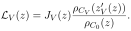
V (z) is therefore read
together with its Jacobian and both covariances:

Searchable transcription

LV (z) = JV (z)ρCV (z′
V (z))
ρC0(z)
.

The density in the denominator belongs to the base measure. Replacing it by the varied density suppresses a real part of the comparison, even if the coordinate map is exact. Its determinant and inverse responses are retained in the detailed calculation.

Activity estimates then transfer local comparisons to reset budgets, and banked contraction gives uniqueness within the fixed recipe and calendar. It does not compare every possible recipe or phase. Path books retain higher jets and insertion transport; the common denominator is kept in omission comparisons. Finally the analytic tail estimates show that omitted insertion terms tend to zero on the same normalized family. Thus the readout at a fixed retained level is recovered with its derivatives and supports, rather than only as an unlabelled scalar limit.

15.1 Omission comparison at a common normalization

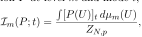
For finest level, period, insertion at level and mode, use throughout

Searchable transcription

R [P(U)]t dμm(U)
Im(P; t) =
ZN,p
,

where is product Haar and 0 is the original finest Wilson partition function. In particular the denominator is not replaced by a new partition function when changes. For positive root weights, the treasury estimate and exact integrated-density identity give

Searchable transcription

|Ik(P; t)| ≤Bk(t) = exp{|Λk|τk + |V |(x + y + 2)}
toll(w, t)
.

At multiply both omitted polynomials by complex and restore); values at one and zero are full and omitted insertions. This bound follows by applying the small-field integral bound to the represented density, bounding its vacuum bill by the treasury, and using the exact identity between the integrated represented density and. The paid analytic estimate makes) holomorphic for = brisk( 2. Transport through the actual retained steps to. Retention preserves served bounds and root weights, and integration is exact. Coefficient extraction commutes with integration as a continuous linear map on the finite-dimensional polynomial algebra. The fixed denominator therefore gives) on the disk. For any bounded holomorphic on radius 2, radius-2 disks centered on [0 1] stay inside it. Cauchy’s estimate gives there; segment integration yields

Searchable transcription

|Y (1) −Y (0)| ≤2B/S.

Thus omission costs at most 2, with root-volume cost at. Analytic paid bounds, retained transport and the root integral estimate are the retained substantive dependencies. For fixed configuration, finite modes, truncated exponentials and local field products make each restored coefficient entire in. Masks and flags are measurable configuration events independent of. The lift retains the finest denominator, omitted pair and actual transport chain. Recovery commutes with coefficient integration and retained steps, preserving the disk bound and Cauchy comparison at that same normalization.

15.2 Integral holomorphy and descending retention

Positive insertion weights make the weighted polynomial norm equivalent to the finite-dimensional coefficient norm. Served envelopes and nonnegative coupling give a finite constant with

Searchable transcription

∥P(z, U)∥≤Y
(|z| < Sj, U ∈Cj).

Probability Haar makes this integrable. Dominated Cauchy-circle integration, or Morera with Fubini, proves integrated-coefficient holomorphy; masks require no configuration differentiability. Retention descends finitely from to. Top scaling spends two support units. At each step the relay identifies first-degree coefficients with the manifest, and Mark feed recovers the next manifest. Parent maps send chosen pins correctly; matching pays occupancy and reweighting; wake data provide local transport tales. The one-step duty bound restores the full support exponent at the next level. Mark-push integrability supplies each stage. This induction explains why the two-unit

expenditure occurs only at the top; it does not accumulate once per step. The finite inventory and one-step duty estimates in the marked-integration chapter establish the inputs to this induction. The retained transport statement has a descending induction with no limiting step. The lift retains this finite chain, manifests and paid envelopes. Recovery commutes with its kernel composition and finite coefficient maps, preserving the common integral majorant and the nonaccumulating exponent cost.

Searchable transcription

For an explicit chain recovery, write Pj→k for the finite composition of the actual retained Mark
kernels and bPj→k for their realized composition. The one-step kernel identity, iterated finitely, gives

Searchable transcription

bPj→kLjP(z) = LkPj→kP(z).

At every level the normalized reader is defined using the same scalar; exact prior and coefficient integration therefore recover

Searchable transcription

bIj(LjP(z); t) = Ij(P(z); t) = Ik(Pj→kP(z); t).

The measurable masks and the constant integrable bound are pulled back together. Thus the holomorphic integrated function, its uniform) bound and its endpoint difference are identical on recovery. The section returns both endpoint insertions. The finite descending retention proof restores the full exponent at each target level, so this commuting chain also preserves the single top expenditure and the 2 omission bound.

15.3 Comparison of varying Gaussian integrals

At a fixed step the fluctuation space has finite dimension For density, physical mean displacement and 0, use. Translation and scalar change of variables give

Searchable transcription

z = g−1(w −tX),
cX(w) = g−DρC(g−1(w −tX)),
Z
A(z) dνC(z) =
Z
cX(w)A(g−1(w −tX)) dw.

Searchable transcription

This retains the Jacobian and transformed integrability for vector-valued A. Covariance bounds give
ρC(z) ≤C0e−τ∥z∥2 uniformly in history and gauge-slice variable. Protected means give ∥tX∥≤B0
by finite coordinate-square summation, and the coupling window gives 0 < u ≤g−1 ≤v. For
r = g−1,

Searchable transcription

1 + ∥r(w −tX)∥≤(1 + v + vB0)(1 + ∥w∥),
e−τ∥r(w−tX)∥2 ≤eτu2B2
0e−τu2∥w∥2/2.

Searchable transcription

The latter follows from ∥w∥2 ≤2∥w −tX∥2 + 2B2
0. A fixed tested-bond face scale lies between one
and K0(1 + ∥z∥). Thus polynomially face-scale-bounded transformed integrands have the common
majorant
C1e−τu2∥w∥2/2(1 + ∥w∥)k,

Lebesgue integrable in finite dimension, uniformly in gauge-slice variable. First apply dominated convergence at each slice point to the transformed integrand differences. Fubini identifies the original Gaussian integrals almost everywhere simultaneously for countably many histories. Their norms are bounded by integrals of the two majorants. The outer gauge-slice prior is a probability measure, so a second dominated-convergence application gives full Gaussian–gauge convergence. The lift retains physical means, scales, densities and the fixed coordinate space. Readout preserves the Jacobian identity and common majorant, transporting both limit passages with the same almost-everywhere scope.

For each fixed prepared datum, define the affine physical-coordinate map. Its recovered measure is exactly

Searchable transcription

If RX is the realized Gaussian reader, then composition of pushforwards gives (TXRX)∗bνX =
cX(w) dw. Thus both histories can be compared on the same physical w space after readout, with
their own retained cX and inverse T −1
X ; the section recovers each inverse formula and its factor g−D.
The common scalar majorant in w is unchanged. For vector-valued integrands the inequality




Z
(Fn −F) dw




 ≤
Z
∥Fn −F∥dw

transports the same dominated-convergence conclusion. The almost-everywhere identifications are retained simultaneously for the countable history indices, and the outer probability prior carries the same integrable constant bound. Hence recovery preserves both integrations and their specified scope without changing the comparison variable or covariance.

15.4 Primitive derivatives and common-draft density comparison

Differentiation under the primitive integral has paid majorant

Searchable transcription

C(1 + (p facescaleK +1))j ≤C(p + 2)j facescaleKj,

since face scale is at least one. Marked derivatives have the same form; undifferentiated marked amplitudes have constant bound. At each fixed gauge-slice point, discrete draft choices are finite and an ultrafilter selects one eventually. Compare histories in that common amended draft, retaining viability, threshold, choices and real and imaginary ingredients. The two-stage dominated-convergence argument then compares ordinary and marked derivatives and amplitudes. Finite reserve products and boundary averages preserve comparison; healthy-support local identities identify these formulas with the actual leaflet and marked-grove germs. This is the Gaussian integral passage used in the single-stream comparison, with all discrete masks retained inside the common draft.

A draft records slice variable, store, boundary choice, selector, scale and width. With the integration point fixed, paid conditions fix the last three, leaving finitely many store/boundary pairs. One fiber belongs to the ultrafilter, since otherwise their finitely many complements would have empty intersection. Viability transfers eventually. This does not assert constancy of continuous slice variables along histories. The common physical fluctuation has restart map

Searchable transcription

zβ(w) =
p
β(w −tX),
tX + β−1/2zβ(w) = w.

Protected-mean and coupling comparisons compare this map. For steered output fields substitute the common smooth steered field for, retaining the analogous exact identity for derivative integrands. The finite Gaussian density is

Searchable transcription

ρC(z) = (
√
2π)−D exp{−1
2 log det C −1
2zTC−1z}.

Covariance comparison, its uniform positive floor and finite inverse and determinant formulas compare every factor. Fixed finite-coordinate density limits are positive, so marginal-density division in local reweighting is legitimate. Principal restrictions inherit the floor and smooth inverse and log determinant. Local correction factors are exactly finite Jacobian times corrected density divided by uncorrected density. Jacobians are products of smooth link steering factors near identity, with chart regularity through the required order. Thus the full correction factor compares through that order; remaining vertices are handled separately. This establishes the density and local change-of-variable factors used in the ordinary and marked integral comparisons. The lift retains discrete drafts, fixed slice points, restart identities, principal marginals and Jacobians. Readout preserves these finite maps and positive denominators, while retained majorants transport derivative integration without discarding masks or complex ingredients.

The local reweighting reader on its fixed tested coordinate set retains the base and varied principal covariances separately:

Searchable transcription

RD(z) = JD(z) ρCV,D(zcorr
D (z))
ρC0,D(zD)
.
(3)

Searchable transcription

Here JD = det Dzcorr
D
> 0 is the original finite steering Jacobian, C0,D is the base restriction, and
CV,D is the varied restriction. Both are positive definite on the common tested coordinates. Change
of variables gives
Z
f(w)ρCV,D(w) dw =
Z
f(zcorr
D (z))RD(z)ρC0,D(z) dz.

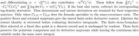
Record the two covariances, the correction map, the Jacobian and their common draft. Positivity of the base density makes the ratio well defined; composition with readout recovers each input and hence this identity exactly, with its original integrability domain. For a smooth family with fixed base, the covariance contribution to the varied log-density is

Searchable transcription

−1
2 tr(C−1
V
 ̇CV ) + 1
2wTC−1
V
 ̇CV C−1
V w,

Searchable transcription

and differentiating w = zcorr
D (z) also contributes − ̇wTC−1
V w.
These follow from
d
dtC−1
V
=
−C−1
V
 ̇CV C−1
V
and
d
dt log det CV = tr(C−1
V
 ̇CV ). If the base also varies, subtract its corresponding
log-density derivative. Thus determinant and inverse derivatives are retained for their respective
matrices. Only when CV,D = C0,D does the formula specialize to the same-covariance ratio. The
positive floors and retained majorants give the stated finite-order derivative control. Likewise the
restart identity is recovered before evaluating derivative integrands.
The finite store/boundary
fiber selected at a fixed slice point is a discrete record and is unchanged by readout. These facts
preserve the pointwise comparison and its derivative majorants while leaving the continuous slice
variable under the same outer integral.

15.5 The protected change of variables and its determinant

The steering factors in the preceding ratio have the following construction. Fix a small positive radius, independent of the later scale delay, on which the logarithm is a left inverse of the exponential through radius 2. Shrink a matrix neighborhood of 1 so that log(exp) is analytic for, and so that for group elements it exponentiates back to exp when These choices follow by continuity on a closed ball strictly inside the original chart. Let the smooth inner-share cutoff, one on, zero for. Define, with this multiplication order,

log(exp Φ ) = det(1+

Outside the cutoffsupport the first expression is identically zero in a neighborhood, so the map is smooth there regardless of the exterior values of the logarithm. On the support, smoothness follows from the chosen analytic chart. At and its derivative vanish, Φ = id, and Compactness of, joint continuity, and the exterior zero identity supply one neighborhood of = 1 on which, uniformly for every

Searchable transcription

∥pM(a)∥< d/2,
∥DapM(a)∥< 1/2,
jM(a) > 0.
(PV2)

Searchable transcription

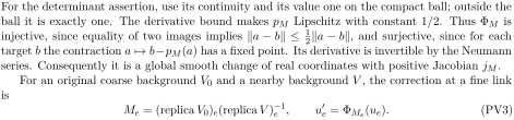
For the determinant assertion, use its continuity and its value one on the compact ball; outside the
ball it is exactly one. The derivative bound makes pM Lipschitz with constant 1/2. Thus ΦM is
injective, since equality of two images implies ∥a −b∥≤1
2∥a −b∥, and surjective, since for each
target b the contraction a 7→b−pM(a) has a fixed point. Its derivative is invertible by the Neumann
series. Consequently it is a global smooth change of real coordinates with positive Jacobian jM.
For an original coarse background V0 and a nearby background V , the correction at a fine link
is
Me = (replica V0)e(replica V )−1
e ,
u′
e = ΦMe(ue).
(PV3)

Searchable transcription

The order matters: for ∥ue∥≤d,

Searchable transcription

exp u′
e (replica V )e = exp ue (replica V0)e.
(PV4)

Searchable transcription

On inactive links the fine slice input remains unchanged. On active links the identity is needed
only where their protecting cutoffs are nonzero.
Those cutoffs imply ∥u′
e∥≤8a tfield.
Choose
the scale delay so that 8a tfield ≤d/2.
Then (PV2) implies ∥ue∥≤∥u′
e∥+ ∥pMe(ue)∥≤d, so
(PV4) applies there. This proves equality of the old and new reconstructed configurations on every
protected read. A cutoffproduct vanishing at the read makes the corresponding term zero. A
nonzero product forces equality on its whole actual footprint. This argument proves the equality
for old activities, atom words, row predictions, sector profiles and their complements individually,
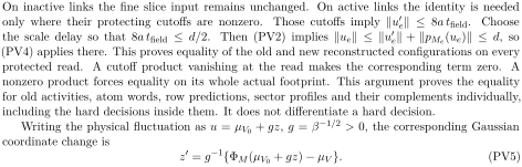
including the hard decisions inside them. It does not differentiate a hard decision.
Writing the physical fluctuation as u = μV0 + gz, g = β−1/2 > 0, the corresponding Gaussian
coordinate change is
z′ = g−1{ΦM(μV0 + gz) −μV }.
(PV5)

It obeys ) exactly, and becomes the identity at. Restrict to the finite set of bond/color coordinates required by the ground. Each link block of (PV5) has derivative ΦΦ; the scalar dilation factors cancel. The coordinate permutation between link/color arrays and Euclidean vectors contributes no absolute determinant. Therefore

Searchable transcription

det Dz′ =
Y
e∈Ilinks
jMe(ue) > 0.
(PV6)

This is a product over tested links, with one color-space determinant per link, rather than one determinant per color component. Let be the principal covariance matrices on, with Gaussian densities . Finite-dimensional change of variables gives for an integrable local function

Searchable transcription

Y
!
ρV (z′(z))
Z
f(w)ρV (w) dw =
Z
f(z′(z))
e
jMe(ue)
ρ0(z) dz.
(PV7)
ρ0(z)
|
{z
}
LV (z)

The denominator is strictly positive at every finite. Both integrals can equivalently be written against the original full Gaussian, since the functions depend only on the indicated marginal and the unused coordinates integrate to one. This proves the local likelihood formula, including its direction and normalization.

Along a smooth coarse field family based at, its finitely many matrices lie in the common neighborhood from (PV2). Differentiation of (PV1) on the compact cutoffball gives uniform finite-order bounds on the displacement and determinant; exterior derivatives vanish or equal those of the constant one. Composition with the coarse family gives a displacement price of the same small order as that family’s motion and a determinant price of order zero. Equations (PV5)–(PV7) then supply the Gaussian score derivatives. The covariance floor and the finite inverse/determinant formulas control the score coefficients. The integrable Gaussian envelopes established above justify differentiation under the integral. Thus a marked entry can remain evaluated on the fixed original fine input: the derivatives fall on its protecting cutoff, on the smooth ordinary vertices, and on The protected equality (PV4) identifies this formula with the original integral on a neighborhood of the base point. This is the mechanism used in the marked primitive comparisons and their product estimates.

Source–readout formulation. The fine configuration is a background-dependent readout of the fluctuation, = Read) = exp() replica . Varying the background at fixed source moves the method’s horizontal operation instead varies while holding the readout fixed, which requires a compensating source motion with Read)) = Read). Equations (PV3)–(PV4) are that horizontal lift,, on the protected domain

1. it exists and is unique there, because the chart logarithm is a left inverse of the exponential;

2. it is extended offthe protected domain by the cutoffto a global diffeomorphism (Lemma 15.1); offthat domain it is not horizontal, and the residual exp(Φ)) replica (exp() replica may differ from the group identity there, which is harmless because every evaluated term carries a protecting cutoff;

3. its Jacobian is (PV6) and its measure-level expression is the likelihood of (PV7), which is the exact price of transporting the Gaussian reference with the background.

Searchable transcription

In the frame realization the replica background is the readout of a raw coarse pair, replica V =
πf(replicaZ(s, B)), and Me is conjugated by the fine frame at the initial vertex of e: Me 7→r−1
x Merx,
ue 7→r−1
x uerx. Since log(exp(Ada) AdM) = Ad log(exp a M) and χd depends on the invariant norm,
ΦM is equivariant, ΦAdM ◦Ad = Ad ◦ΦM, and jM is invariant. The horizontal lift, its determinant
and LV are therefore fibre constants, recovered exactly on the identity-frame section.

Lemma 15.1. Under (PV2), Φ is a global smooth diffeomorphism of the real color space with positive Jacobian

Proof. The injectivity, contraction-surjectivity and Neumann-series argument immediately following (PV2) proves the claim, including positivity of the determinant. This is the same finite map; no second extension is chosen for the source–readout formulation.

The exactness class is exact recovery on the protected domain and an explicitly retained residual offit; what is supplied as realization data is the cutoff and the protected radius, and what is derived is the horizontal lift, its uniqueness there, its Jacobian and the likelihood.

15.6 Finite-window covariance and common activity comparisons

The form matrix evaluates selected physical rows on fixed coordinate impulses. Selection means the row base lies outside the store’s fixed six-radius interior. Unselected rows vanish in both histories; selected rows compare through the required derivatives by physical-row comparison. The plate is their Gram matrix plus fixed dormant diagonal, so finite multiplication compares its entries. Each covariance column uses its fixed reference-frame window. Principal restrictions inherit the positive floor; smooth finite inversion with the common inverse bound compares derivatives. The scalar density proof above consequently rests on finite inverse matrices with a common lower eigenvalue bound. Outside-window entries remain zero. Embed columns and symmetrize to recover the actual reference covariance. Protected means use these columns and local bills, so their comparison supplies restart with coupling comparison. The inputs remain the stationary and local nonlinear row/bill estimates. This retains the column-window construction and does not replace it by the full plate inverse.

At fixed level and physical period use one normed presentation with fixed dictionary, supports and threshold; its completion is only for limits. Actual retained histories lie in the original space. The norm bounds a uniform absolute evaluated budget by: sum regular masses over anchors

and forced masses by chosen sites of nonempty inventories. At a fixed period one may take to be the number of sites times the corresponding anchored budget constant. The canonical envelope

Searchable transcription

q(a, i) = sup
U
|F(a, i, U)|

is finite, nonnegative and summable with total at most. Linearity gives ). For Cauchy, choose with2 later, and a finite label set controlling tails of by2. Subadditivity gives every later tail at most. For Cauchy with vanishing norm difference,

Searchable transcription

|F(an, i, U) −F(bn, i, U)| ≤q(an −bn, i) ≤C∥an −bn∥

uniformly in configuration. Fixed masks keep regular evaluation linear; actual inventories and uniform tails are retained. Escaping subsequences of a single Cauchy activity sequence compare, since their norm difference tends to zero by the Cauchy criterion; so do real couplings. Isometric completion convergence suffices for the original presentation’s Cauchy property. Hence all incoming regular, incoming forced and outgoing forced comparisons required by the two-history transfer argument follow from the common activity Cauchy sequence. The two envelope families also have the uniform tail property just proved.

Normalized scalar coordinates lie in fixed compact intervals at each level. Countable-product compactness gives a diagonal escaping subsequence with all scalar limits; fixed-scalar construction then gives activity and intermediate convergence. Repeat on every escaping subsequence. Comparison of banked limits at the same bottom coupling, at level zero, identifies scalar limits; the subsequence criterion gives full scalar convergence, then full activity convergence. That comparison is proved in Subsection 15.11; compactness is used only to obtain the candidate limits. Winning trajectories have the same prescribed bottom coupling ̄ at level zero. Finite-horizon alignment

identifies their stationary paths and actual retained activity presentations, supplying the original common-choice Cauchy sequences. The lift retains fixed windows, masks, presentation norms and subsequence comparisons. Readout preserves the column construction and uniform envelope bounds, and its isometric recovered presentation transports these Cauchy and limit statements with their stated uniqueness dependency.

Explicitly, let include the fixed window for covariance column into the physical coordinate space, and let be that column’s coordinate vector in the window. For physical plate, the column reader and symmetrization are

Searchable transcription

vj = Ej(E∗
j QEj)−1ewin
j
,
V = (vj)j,
C = 1
2(V + V ∗).

All adjoints here use the recorded physical Euclidean metric. Realization recovers and the positive principal restriction before inversion; section recovery therefore gives these same columns and covariance, with zero exterior entries. Smooth finite inversion transports the stated derivative comparisons on the common positive-floor domain. For activity evaluation define )). Surjectivity provided by the section gives the exact envelope equality

Searchable transcription

sup
z |F Z(a, i, z)| = sup
U
|F(a, i, U)| = q(a, i).

Thus the recovered presentation has the same canonical envelopes, uniform finite-label tails and norm-controlled differences. This preserves the Cauchy comparisons and their completion limits together with the retained banked-limit uniqueness dependency.