The common continuum hierarchy · Part 2

symmetry has not yet been established, use (CVP1) instead. This supplies a uniform bound at every cutoffand the required exact symmetries on the admitted tail.

The projection maps are therefore idempotent and uniformly bounded before extraction. Their limits are idempotent as well, at each fixed period and in the outer limit. Their kernel dimensions stabilize in both limits. Indeed, if are idempotents and 1, the map sends ker into ker injectively: if and = 0, then forcing = 0. Interchanging gives equal kernel dimensions. The physical detector estimates identify the limiting kernel with the exact equation-null space, rather than merely bounding its dimension. The transported insertion comparison shows that a label in this kernel has vanishing separated smeared correlations: its discrepancy has a uniform separated bound tending to zero, and the step-function integral argument gives the same vanishing for every compact separated test.

Conversely, the finite full-rank detector pairs separate the quotient. A label with zero continuum correlations against every spectator has zero detector readings, hence lies in the limiting kernel. Thus continuum-null labels of degree = ker (CV2)

The quotient is finite dimensional, carries the real and signed-motion structures preserved by and is the same quotient used for the detector normalization and subsequent differentiation.

The derivative construction removes the coordinate-projection restriction on the raw table. Transport the finite differences to this quotient using their retained coefficient estimates. Their limits agree with the raw table on generic tuples. The local Taylor and next-difference argument proved earlier identifies their derivatives and extends them smoothly across coordinate ties, as long as no two full four-dimensional positions coincide. The generic set is dense there, so two continuous such extensions must agree. This gives the smooth table with the original as its fixed-period tables and the same separated smeared limits. No pointwise assertion at a coordinate tie is obtained from raw compactness alone.

In the present construction the full fixed-volume mesh limits were already established by the two-level Cauchy argument. The auxiliary mesh subsequence just used therefore converges to those same. To see explicitly that this restores the required smeared order, fix a token word and one compactly supported separated test. For each suitable period, let) be its lattice smeared moment. The full-mesh result gives. The extracted table gives, along its mesh subsequence), a limit), followed by the stated volume limit of Cofinality of also gives). Uniqueness of a complex limit therefore identifies ) at each suitable. Substitute this equality into the retained volume-limit identity. The result has the full mesh order followed by precisely the same volume subsequence as the final table. This argument restores the smeared convergence assertion; it does not claim that every auxiliary structure originally extracted on a mesh subsequence has been extended to all meshes.

Finally, countably many further stages can be imposed without combining incompatible choices. If each successive order refines its predecessor, take its diagonal mesh and period sequences separately. For a nested sequence of strictly increasing sequences, the diagonal) is strictly increasing: writing, one has + 1. For every fixed stage, the tail of lies in the range of. Apply this to mesh and period orders. Every eventual bound and every retained limit from any fixed stage survives on the resulting diagonal order. This is why the hierarchy, quotient, numerical limits and later comparison services can all be attached to the same extracted table.

The calibrated equation image and its silent representatives

We specify the finite-cutoffchange of coefficients used in the preceding projection construction. This also explains why its kernel directions are silent in continuum tests. Fix a degree, its coefficient frame, and a second sound local section , such as the marked equation section. Write for the coordinate vectors and1 for the fixed cost of signed motions and coordinate decomposition in this frame. The local insertion transport constructs columns satisfying

Searchable transcription

|ej −uj|coeff≤(2c2)−1.
(CVR1)

The columns are combined by the signed and conjugate averaging already used for local sections, rather than by an unsymmetrized matrix. Explicitly, if) are the averaged coordinates of the inverse motion of, then

Searchable transcription

Px =
X
s,j
χs,j(x) suj,
x =
X
s,j
χs,j(x) sej,
X
s,j
|χs,j(x)| ≤c|x|coeff.
(CVR2)

Here a conjugating motion conjugates the coordinate as well, so the combined map is complex linear. The fixed motion bound is. Subtract the two sums and apply (CVR1):

Searchable transcription

|x −Px|coeff≤1
2|x|coeff,
|P −1y|coeff≤2|y|coeff.
(CVR3)

Indeed the first inequality makes injective; finite dimensionality makes it surjective, and applying the first inequality to gives the second. These bounds hold uniformly in the period on the eventual mesh tail.

For precision about the purchase of (CVR1), putstencilstencil, where is the original section. At stage, write for the support exponent, for the number of columns, and0 for the purchased derivative-credit bound of . The transport estimate gives

Searchable transcription

L1/8
N−1|ej −uj|coeff≤2(1 + qN)YN,
YN = 2 + e81hN (bN + qN + 2|X|).
(CVR4)

Searchable transcription

The delayed length requirement is precisely 2(1+qN)YN ≤L1/8
N−1/(2c2), which proves (CVR1). It is
bought together with bN ≤bβN, not inferred from a limit after selecting the columns. The common
error price can be taken to be

Searchable transcription

EN = 4(1 + qN)YN + e81(hN+2)ZNζd,N/uN,
ZN = (aV + 2aT )
X
j
θ−fj
N ,
(CVR5)

Searchable transcription

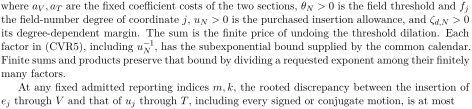
where aV , aT are the fixed coefficient costs of the two sections, θN > 0 is the field threshold and fj
the field-number degree of coordinate j, uN > 0 is the purchased insertion allowance, and ζd,N > 0
its degree-dependent margin. The sum is the finite price of undoing the threshold dilation. Each
factor in (CVR5), including u−1
N , has the subexponential bound supplied by the common calendar.
Finite sums and products preserve that bound by dividing a requested exponent among their finitely
many factors.
At any fixed admitted reporting indices m, k, the rooted discrepancy between the insertion of
ej through V and that of uj through T, including every signed or conjugate motion, is at most

Searchable transcription

Cd,m,kENe−sN/8,
Cd,m,k = exp{(am/ak)4τk + 5} a−d
k
ζd,k/4esk/8.
(CVR6)

Here is the explicit vacuum treasury derived in the denominator estimates above. These are fixed finite constants after the reporting indices are chosen. Expand any subexponentially priced coefficient row by (CVR2). The finite number of terms and their subexponential coordinates, together

with (CVR5), absorb at most eventually. Thus the entire discrepancy has rooted bound tending to zero, with a remaining exponential factor. Its fixed stencil, gauge invariance and continuity make it eligible for the separated spectator product and smearing argument below. Let be the terminal coefficient isomorphism and the marked embedding of free labels into terminal coefficients. The calibrated equation image is exactly

Searchable transcription

KN,p = T PT −1B(Id).
(CVR7)

If, set. Then). The actual insertion through with coefficient is therefore exactly zero against physically separated spectators on a sufficiently fine mesh, by the local marking identity. The uniform radius for that assertion was proved by the finite-basis maximum in the equation-lift construction. Formula (CVR3) preserves the subexponential price of , and (CVR6) compares this exactly silent insertion with the original insertion of. Consequently every subexponentially priced row in (CVR7) tends to zero against every separated test. This is the kernel cancellation used in (CV2) and (QD3); it follows from the actual calibrated map and a local identity, rather than from dimension counting alone.

Inclusions and derivatives on the same physical quotient

The differential system is constructed using all spectator tests on this quotient. Let be the finite coefficient space and the null subspace in (CV2). A test reading means: put the distinguished label at any chosen slot, put arbitrary other labels in all remaining slots, multiply the correlation by a smooth compactly supported test whose support lies in the separated configuration space, and integrate. Denote it by), including the spectator data in. The family of all these linear functionals has common kernel. For a smooth table this follows from uniqueness of continuous kernels as distributions on the open separated set; a nonzero value has a neighborhood and a compact bump detecting it.

At finite mesh, a derivative insertion is the actual forward difference

Searchable transcription

δaIb(o) = a−1
N {Ib(o + ea) −Ib(o)}.
(QD1)

In the finite torus sum, translating the distinguished summation variable gives the exact summationby-parts identity

Searchable transcription

a4n
N
X
r
ψ(aNr) ⟨δaIb(ri) spectators⟩= a4n
N
X
ψ(aNr −aNei,a) −ψ(aNr)
aN
⟨Ib(ri) spectators⟩.
r

(QD2) Translation is a permutation of the finite torus, so this is true even at its seam. Once the physical period contains the compact support and its one-step thickening, both potentially nonzero terms have their actual cover coordinates. Taylor’s theorem makes the test quotient converge uniformly to, on one fixed separated compact. The separated correlation bound controls the remainder in the cell integral. Take the mesh limit at that fixed suitable period first, and then the retained volume limit. This proves the derivative test limit in the same mesh-then-volume order as the hierarchy; no uniform count of lattice points over all periods is needed.

Searchable transcription

The coefficient approximations used for both inclusion and (QD1) have subexponential top-
coordinate cost: for every ε > 0, their pullback to the terminal frame is eventually bounded
by exp(εsN), where sN is the calendar scale. For bounded reference coefficients this follows by
multiplying the backward column bounds: their logarithm is P
i<N log Ci.
The calendar gives
log Ci ≤ε log Li/2 after a fixed level, so the tail is at most ε(sN −sk)/2; the finite head is absorbed

into The relay estimates extend this cost statement to the actual inclusion and finite-difference approximations.

Here is why their errors vanish against every test. A local rooted discrepancy bound with reporting spacing chosen arbitrarily small after fixing its requested tolerance, gives a separated correlation bound. Choose that reporting spacing below the physical separation, place the spectator insertions in distinct cells, and apply the reflection-positive product estimate, leaving the discrepancy in its own cell. Its compactly smeared sum is the integral of a step function, bounded by this quantity times the test supremum and the volume of one fixed enlargement of its support. Hence it tends to zero. This also applies to an exactly silent separated remainder with zero bound.

One must control approximations before assuming their coefficients bounded. Write for the finite projection and for an approximating coefficient. Normalize its null remainder by

Searchable transcription

zN,p = xN,p −PN,pxN,p
1 + ∥PN,pxN,p∥.
(QD3)

It lies in the finite projection kernel. The normalized projected part has norm at most one and therefore the subexponential cost just proved. Multiplication by the reciprocal denominator costs at most one, and subtraction preserves subexponential cost by spending2 on each summand. The relay’s equation cancellation then gives0 for every test. This is precisely the normalized remainder required by the detector argument: it proves boundedness and recovery of the projected limit using the stable finite detector, without presuming boundedness of the unprojected approximant. The detector identifies its limiting responses with one vector in

Apply this recovery to an inclusion from horizon to, and to (QD1) from to + 1, first on a fixed basis of. Choose representatives of the recovered vectors and extend linearly. This gives linear maps and satisfying, simultaneously for all spectator tests, (QD4)

The same approximating coefficient family is used for every spectator; separate choices for different tests would not define a field. If, the right sides of both equations (QD4) vanish for every test, including the differentiated test, which still has compact separated support. Thus and. The quotient maps (QD5)

are consequently independent of the chosen representative. Their pointwise kernel identities follow from (QD4): inclusion gives equality of two continuous kernels, and integration by parts gives the ordinary derivative of the smooth kernel. Integration by parts is legitimate on the separated open set because the test support is a compact subset of that set. Extend the product of test and kernel by zero outside; it is smooth with compact support, so its total directional derivative integrates to zero.

Faithfulness against all spectators now proves every compatibility law. Inclusion is injective, since its zero class has exactly the same readings as its input. Inclusions compose and the identity inclusion is the identity, since both sides have identical readings. Differentiation commutes with inclusion, because it differentiates the same smooth kernel in either horizon. Two derivatives commute by the ordinary mixed-derivative theorem. The derivative of the unit is zero: the unit removes its insertion slot and the resulting kernel is independent of that coordinate. Permuting insertion slots transfers these identities from the distinguished first slot to every slot by the linear permutation chain rule.

Finally conjugation commutes with real directional differentiation. For a signed orthogonal motion, its coordinate derivative transforms by

Searchable transcription

∂b(f ◦s) =
X
a
sab(∂af) ◦s.
(QD6)

Apply the already established reality and signed covariance identities to the kernel, differentiate on the separated neighborhood, and use faithfulness again. It follows that the quotient inclusions commute with both symmetries and that the quotient derivatives obey (QD6). This establishes the differential structure on the actual null quotient used in reconstruction, with no extra representativedependent operation.