Marked integration and the coupling reset · Part 2

One direction follows from shortest-path distances and the least-parent choice. Conversely, containing the stem gives a path of assigned length from the root to every vertex, while the upper constraint prevents any shorter path; hence these are the graph’s actual distances. The second constraint and injectivity of the order give the same least preceding-level neighbor. Thus the breadth-first parent is again. These intervals partition all connected subgraphs of the original graph. If stem() contains an edge, toggling it pairs every graph in the interval with one of opposite parity. The interval sum vanishes. If there is no such edge, its sum has absolute value one. Summing interval bounds proves precisely the rooted spanning-tree bound on the absolute connected coefficient.

Passing from numbered trees to distinct connected sets

The same forest estimates also bound distinct-set expansions. For a distinct label set of size parent map on, and each bijection, relabel the parent map and its activities by that bijection. The resulting numbered forest determines all three objects: its label range is, its label assignment determines the bijection, and transport back through that bijection recovers the parent map. This assignment is injective. There are exactly! bijections; all have the same product weight divided by!. Their sum is therefore the unnumbered product weight, with no factorial left. Restricting the numbered forest sum to this injective image proves the distinct-parent-map estimate and its geometric size tail.

A finite overlap-connected set whose union meets can be rooted at the external support (x). Connect the root to labels whose supports contain, and use a breadth-first spanning tree of the resulting connected graph. The sum over all parent maps includes this one, so it dominates that set’s nonnegative product weight. For the stronger sitewise prefactor, instead choose one label containing as an internal root, charge its activity to the site’s budget, and use the internal-root forest estimate for the other labels. Summing over all possible roots only increases the bound. Numbering the distinct nonroot labels cancels their factorial exactly as above; allowing the root label once more among nonroots in the majorant is harmless. Consequently the distinct connected-set sum rooted at, with the actual union support weight, is bounded by) under the readiness assumptions. This is the distinct-set input used in the positive-multiplicity restoration argument.

Cluster logarithms with repeated occurrences

Let (R(i,j)) be a symmetric incompatibility relation with (R(i,i)) for every label. Letbe its support, with incompatibility implying intersecting supports. For real activities, the hard-core gas is

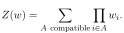
Searchable transcription

Z(w) =
X
Y
i∈A
wi.
A compatible

The empty subset contributes one. In contrast, its logarithm uses ordered occurrence tuples ), permitting repeated labels. Form the graph of incompatible occurrence pairs and define

Searchable transcription

n
Y
φ(z) =
X
(−1)|E(H)|,
L(w) =
X
X
1
n!
z∈In
φ(z)
j=1
wij.
H connected
H⊆incompatibility graph
n≥1

For one occurrence the connected graph has no edges and coefficient one. Equal labels at distinct occurrence positions are incompatible. This is essential to the logarithmic identity even though the gas itself is indexed by distinct-label subsets.

The absolute estimate uses cancellation inside. Breadth-first exploration partitions connected subgraphs into intervals with one fixed spanning tree as lower endpoint and an allowed edge set as upper endpoint. In each interval, if an optional edge exists, toggling that edge is a sign-reversing involution, so the alternating sum is zero. Otherwise the interval contains only its tree and its absolute contribution is one. Hence is bounded by the number of compatible rooted spanning trees. Opening the absolute value before the connected-graph sum would lose this estimate.

Here is the resulting root accounting. Put) = coverNumber), take and suppose

Searchable transcription

X
i:x∈Xi
|wi|e(a+δ)cB(Xi) ≤γ,
0 < q < 1,
4(2B + 1)4γ
δ
≤q.
sup
x

Searchable transcription

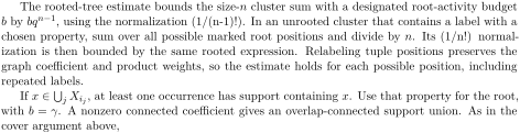
The rooted-tree estimate bounds the size-n cluster sum with a designated root-activity budget
b by bqn−1, using the normalization (1/(n-1)!). In an unrooted cluster that contains a label with a
chosen property, sum over all possible marked root positions and divide by n. Its (1/n!) normal-
ization is then bounded by the same rooted expression. Relabeling tuple positions preserves the
graph coefficient and product weights, so the estimate holds for each possible position, including
repeated labels.
If x ∈S
j Xij, at least one occurrence has support containing x. Use that property for the root,
with b = γ. A nonzero connected coefficient gives an overlap-connected support union. As in the
cover argument above,

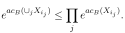
Searchable transcription

eacB(∪jXij ) ≤
Y
j
eacB(Xij ).

Thus, summing sizes + 1, the absolute logarithmic terms whose support contains including their actual union support weight, have total at most

Searchable transcription

γqm
1 −q.

Searchable transcription

Summing root bounds over all sites gives absolute convergence of L at fixed torus, with total
at most |Λ|γ/(1 −q). The rooted-tree estimate and its breadth-first interval construction are the
remaining combinatorial ingredients behind this bound; the occurrence/root normalization and
transfer to the union support have been made explicit here.
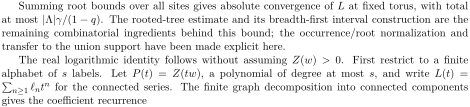
The real logarithmic identity follows without assuming Z(w) > 0. First restrict to a finite
alphabet of s labels.
Let P(t) = Z(tw), a polynomial of degree at most s, and write L(t) =
P
n≥1 lntn for the connected series. The finite graph decomposition into connected components
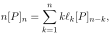
gives the coefficient recurrence

Searchable transcription

n
X
n[P]n =
k=1
klk[P]n−k,

obtained by designating one occurrence, choosing its connected component and then the remaining graph. The binomial choices of positions and the component factorials give precisely these coefficients. The absolute cluster bound gives. Choose 1 with 1; both (L(t)) and its differentiated series converge uniformly on compact subsets of ((-u,u)), by the summable

Searchable transcription

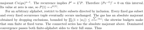
majorant Cn(qu)n−1. The recurrence implies P ′ = L′P. Therefore (Pe−L)′ = 0 on this interval.
Its value at zero is one, so P(1) = eL(1).
For an arbitrary alphabet, restrict to finite subsets directed by inclusion. Every fixed gas subset
and every fixed occurrence tuple eventually occurs unchanged. The gas has an absolute majorant
obtained by dropping exclusions, bounded by Q
i(1 + |wi|) ≤e
P
i |wi|; the sitewise budgets make
that sum finite at fixed torus. The connected series has the absolute majorant above. Dominated
convergence passes both finite-alphabet sides to their full sums. Thus

Searchable transcription

Z(w) = eL(w) > 0,
log Z(w) = L(w).

This also applies after removing all labels incompatible with a specified forced set: the absolute activity budgets only decrease.

Primitive marked integrals and averaging over local tree choices

The primitive activity attached to a marked team is an actual integral. A team is a finite collection of real local leaves with distinct dictionary keys; its weight is the product of their bounds and its ingredient the product of their functions. For a fixed coarse configuration and local tree choice, first choose a permitted flag sector, a local block layout, and a finite list of warning and regularexponential selections. Their union is the molecule address. The marked integrand is the product of the team’s paid ingredients and the selected local vertex factors; it is set to zero unless all of the team’s keys occur in. Its primitive coefficient is its integral over the tree-gauge variables and the Gaussian fluctuation variables. The Gaussian measure has the covariance and density already attached to that same local tree choice. Sector selectors and all eligibility tests stay inside this integral.

More explicitly, if denotes that local data, the sector, and) its selected integrand, set

Searchable transcription

Z
IX,k,p(h, z) dνX(h) dγX(z).
aX,k(p) = 1approved(X,k)

The full primitive coefficient averages these values over the finite boundary choices for the layout of; it is zero for a disallowed layout. Its scalar prefactor is the original local overhead. The local vertex and integral estimates are developed in the packet, non-packet and warning arguments below.

Searchable transcription

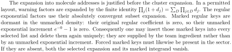
The expansion into molecule addresses is justified before the cluster expansion. In a permitted
layout, warning factors are expanded by the finite identity Q
j(1 + dj) = P
Q
j∈D dj. The regular
D
exponential factors use their absolutely convergent subset expansion.
Marked regular keys are
dormant in the unmarked density: their original regular coefficient is zero, so their unmarked
exponential increment e−0 −1 is zero. Consequently one may insert those marked keys into every
selected list and delete them again uniquely; they are supplied by the team ingredient rather than
by an unmarked exponential increment. Forced marked keys must likewise be present in the sector.
If they are absent, both the selected expansion and its marked integrand vanish.

The resulting address assignment records the layout, sector, warning list and regular list. It is injective on permitted data and has an explicit inverse obtained by reading these pieces from. Thus each nonzero molecule occurs with exactly the specified coefficient, and disallowed molecule addresses contribute zero. The summable activity majorant bounds the integral norms of these terms by the team’s weight times the product of the unselected primitive tariffs. This gives a summable series of integrable terms. Fubini and the theorem on integration of a series with summable integral norms therefore give

Searchable transcription

X
p
overheadX aX(p) = P(team density)(U).

This is the primitive team expansion. In Gaussian coordinates the change of measure is explicit: . The transformed integrand contains that same and its tribute prefactor, so the Gaussian integral agrees with the original local fluctuation integral by substitution of the density. No independent Gaussian approximation is made in this identity.

To obtain compatible products of primitive coefficients, average over independent local tree choices at coarse sites. A molecule’s integral depends only on the tree choices in its enlarged ground support. To prove this locality, project the fluctuations to the finite coordinates needed by that ground. Two local data sets agreeing there have the same projected covariance. Their Gaussian pushforwards under the coordinate projection are therefore the same measure. The integrands depend only on those projected coordinates and agree on each fiber, by their local footprint formulas. Their integrals coincide. The same argument applies to the gauge variables through their local measure-preserving coordinate maps. Thus changing exterior tree choices leaves the molecule coefficient unchanged.

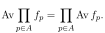
Compatible molecule grounds are disjoint. For functions of independent finite choices, each depending only on its ground, finite product averaging gives

Searchable transcription

Av
Y
p∈A
fp =
Y
p∈A
Av fp.

This follows by factoring the finite sum over assignments on disjoint coordinate sets; unused coordinates contribute one. The local scalar overhead is invariant under the tree choice. Averaging the team expansion consequently yields the product of the averaged molecule coefficients with the original compatibility and inventory conditions.

Finally expand a finite leaf inventory into tickets with distinct keys. On a compatible set of molecules, every chosen leaf key lies in exactly one molecule; selecting it there gives a unique global ticket, and conversely a global ticket restricts uniquely to each molecule. Multiplication of the leaf amplitudes factors over this partition. Hence the product of primitive marked molecule sums is exactly the ticket sum of the team’s compatible product. Finite linearity of the Mark integral then proves

Searchable transcription

X
!
X
!
X
A compatible,permitted
overhead
Y
Y
Y
i∈D
vi aD(p)
= P
i∈D
vi teamDensityD
(U).
p∈A
D ticket
D

The primitive-integral bounds and support-hit estimates in the nonlinear and marked-integration chapters give these summable integral-norm and footprint bounds. The address regrouping, Gaussian marginal comparison, independent tree averaging and ticket factorization show how they produce the literal Mark expansion used in the gas/log argument.

Fusing attached logarithms into the forced dictionary

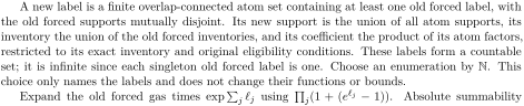
The dictionary fusion used twice in the coarse construction has an explicit formula. Let the old forced labels be, with supports, nonempty inventories, and coefficients). Let attached logarithms) have nonempty supports, and suppose= 0 only if meets the configuration’s flagged set. Both families have summable uniform envelopes. Form the disjoint atom alphabet of old forced labels and attachments, with factors

Searchable transcription

hf,i = Ki(U),
ha,j = elj(U) −1.

Searchable transcription

A new label is a finite overlap-connected atom set containing at least one old forced label, with
the old forced supports mutually disjoint. Its new support is the union of all atom supports, its
inventory the union of the old forced inventories, and its coefficient the product of its atom factors,
restricted to its exact inventory and original eligibility conditions. These labels form a countable
set; it is infinite since each singleton old forced label is one. Choose an enumeration by N. This
choice only names the labels and does not change their functions or bounds.
Expand the old forced gas times exp P
jlj using Q
j(1 + (elj −1)).
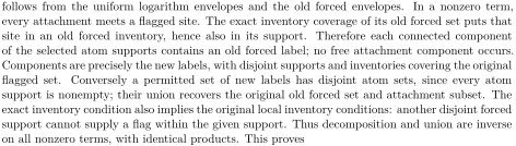
Absolute summability

Searchable transcription

follows from the uniform logarithm envelopes and the old forced envelopes. In a nonzero term,
every attachment meets a flagged site. The exact inventory coverage of its old forced set puts that
site in an old forced inventory, hence also in its support. Therefore each connected component
of the selected atom supports contains an old forced label; no free attachment component occurs.
Components are precisely the new labels, with disjoint supports and inventories covering the original
flagged set. Conversely a permitted set of new labels has disjoint atom sets, since every atom
support is nonempty; their union recovers the original old forced set and attachment subset. The
exact inventory condition also implies the original local inventory conditions: another disjoint forced
support cannot supply a flag within the given support. Thus decomposition and union are inverse
on all nonzero terms, with identical products. This proves

Searchable transcription

Gasnew(U) = Gasold(U) exp
X
j
lj(U).

The regular dictionary and its original coefficients remain the regular part of the fused representation. The attached logarithm is consumed only through the displayed exponential and the new forced factors. Gauge invariance and measurability pass to finite products and measurable eligibility indicators. Locality uses the union support. Widening a dictionary beforehand is simply an injective placement of its old labels in a universal dictionary with zero coefficients at all unused indices. It preserves the gas and the regular-log sum by reindexing the absolutely convergent families.

The fusion estimate for switched coefficients follows from the distinct-component forest bound already proved. Suppose the old switched forced coefficients have paid sitewise budget at support exponent (s+1), and the fixed attached logarithms have envelope budget there. Choose 0. Assign inflated envelope to an old forced label and envelope 2 to an attachment with 1. The latter bound is justified by

Searchable transcription

|ex −1| ≤2|x|
(|x| ≤1),

which is used on the source’s smaller admitted logarithm range. The combined sitewise budget is

Searchable transcription

γ = eκB0 + 2w0.

Each new connected label contains an old forced atom. Undoing its inflation supplies at least ; every other undone factor is at most one. Thus its paid envelope is bounded by times the product of the inflated atom envelopes. Its eligibility indicator is independent of the switches and does not increase the price. If1, the earlier connected-component forest estimate, spending one supportexponent unit, bounds the new sitewise paid budget at exponent by

Searchable transcription

e−κ(eγ −1).

The selected payment inequalities require this quantity to fit the requested output allowance. This proves transfer of the paid switching family through each fusion. The family’s unmarked value is the fused unmarked coefficient by the same formula. An exterior-switch silence identity passes through fusion term by term: if an atom’s union support omits the required parent site of a switch, each factor is unchanged on erasing that switch; so is their product and its eligibility indicator. These facts supply the value, price and scope properties needed after the two actual coarse dictionary changes.

The scalar normalization needed after these fusions is an equality of exponents, not a comparison of partition functions. Let) be the intermediate frozen exponent, let) be the coupling-reset receipt, let be its coefficient, and let) be the attached-log sums consumed by the two fusions. The path reset gives

Searchable transcription

Efinal(U) + L2(U) = E0(U) −αR(U).

The unmarked local integral normalization gives

Searchable transcription

exp{E0(U) + L1(U) −αR(U)} = overhead(U)Z0(U).

Combining these equations and the exponential addition law proves

Searchable transcription

eEfinal(U)eL1(U)eL2(U) = overhead(U)Z0(U).

In particular both sides use the same unmarked local gas that appears in the switched formula. Subtracting its logarithm in the switched regular increment cancels precisely this normalizer. The path-reset identity and unmarked local normalization proved in this chapter retain the stationary path and vacuum choices used here.

The coupling-reset exponent identity

The reset changes the represented coupling and compensates that change by explicit local counterterms. The total density is preserved by the displayed exponent identity. Its projected coefficient is read from the affine Hessian with the source’s chosen normalization. A probe value is a different operation and is not silently identified with that projection.

We now specify the reset in the scalar identity. Let be the source on a listing, let be the same path family used in the kinetic energy, and let fix the threshold, support scale and Taylor order. All masks below are the actual healthy-field masks at that threshold. Write ∆=(read and let be the already committed loop coefficient. The new coupling and vacuum scalar are

Searchable transcription

X
β′ = β + α + ∆,
τ ′ = τ −
1
|Site|
i
logReadi(v; 1).

The receipt) is the averaged sum of the masked plain low path terms, with their original paths. It is not obtained by changing paths to match a later choice. The regular-source decomposition separates each log read into its value at the identity, a local projected payout, a fault, and a masked rebate. Absolute summability of the original paid activities bounds these four series respectively by the original total bill and fixed multiples of it. Summing

Searchable transcription

the payouts first at their anchor sites gives ∆P
o headsp(o, U), by the calibrated projection identity.
Consequently

Searchable transcription

additivep(readX(v); U) =
X
i
logReadi(v; 1) + ∆
X
o
headsp(o, U)
−
X
i
dusti(U) +
X
i
untaggedi(U).

Searchable transcription

The projected-payout identity uses the simple-group projection hypothesis and the stipulated period
n > 20.
There are also low and high path corrections. Denote their averaged sums by F∆and Hα,∆,
and the low loan sum by Lα,∆. Their defining termwise identities, summed with the same masks,
are
(α + ∆)KR + F∆+ Hα,∆= αR + ∆
X
o
headsp(o, ·) + Lα,∆.

Indeed the true kinetic base is the sum of live low terms and high summits. The high correction is minus + ∆times the summit, so those terms cancel. For each low term its defining loan identity reads + ∆) live + fade maskedPlain + ∆sketch + loan

The sketch sum is the head sum. The low live, masked plain, proxy and fade series are absolutely summable by the path bounds; this identity then also proves summability of the loans. The high summit series is absolutely summable as well. Averaging over the finitely many seats preserves these properties. Hence the cancellations are valid equalities of convergent sums.

The reset dictionary’s additive sum is the untagged sum plus; its attached logarithm is the dust sum plus. Substitution into the representation exponentSiteinChannels( additive, followed by the two displayed identities and the channel decomposition, gives

Searchable transcription

Ereset(U) +
X
i
logi(U) = Efrozen(U) −αR(U).

This is the path-reset identity used above, including its constant term and signs. Exponentiation gives the same identity for unnormalized evaluators. It holds even when the activity gas vanishes, since the gas multiplies both sides and is never divided out. The subsequent dictionary fusion absorbs the attached-log exponential by the already established fusion identity. The lower-level projection, live-base and loan formulas supply the mathematical content of this reset decomposition and must retain the same threshold and paths.

Gauge invariance at the flat germ

Let(increment(1)). Regularity gives a twice continuously differentiable germ at Constant gauge transformations act there by the linear mapAd, because exponentiation commutes with conjugation. Hence(0), restricted to a single edge’s color space, is an invariant linear form. Such a form vanishes. Indeed differentiating invariance along exp() shows it kills every bracket []. Its kernel is an ideal; simplicity makes this kernel zero or the whole algebra. The zero case would make the form injective and force all brackets to vanish, contradicting non-abelianness. Summing single-edge directions proves(0) = 0. Twice differentiating the same constant-gauge identity proves adjoint invariance of

For a color-valued site field, let (). Gauge the link exponential of by the site elements exp()), and take its local logarithm. This defines a smooth chart near zero with

The derivative follows by differentiating the three factors on each link: the contributions are The local logarithm recovers the gauged configuration near the identity. Gauge invariance gives). Differentiate this equality in directions (0 1) and 0). In the second chain rule the term involving is multiplied by(0) = 0, while the right side has no-dependence. Thus

Its symmetric counterpart follows from symmetry of the second derivative. Locality implies that Hessians agree when the tested direction fields agree on the support: first compare their diagonal exponential lines, then polarize. These arguments concern smooth unmasked germs throughout.

The color-bilinear assertion used below also admits a direct finite-dimensional proof. If is adjoint invariant, differentiation gives Its antisymmetric part satisfies). Cycling this relation and using bracket antisymmetry makes this value equal to its negative, so it is zero. For fixed, the linear form) kills brackets, and the kernel argument above makes it zero. Hence is symmetric.

Representby a self-adjoint real operator. Invariance and skew-adjointness of the adjoint action give]. A nonzero real eigenspace of exists by the finite-dimensional spectral theorem and is an ideal by this commutation identity. Simplicity makes it the whole color space. Thus and. Skew-adjointness here follows directly by writing the color inner product as the real matrix trace and cyclically moving the commutator factors. This proves the invariant-bilinear-form input without an assumption about a complex or infinite-dimensional color representation.

Reduction of affine tests to constant curl

Use centered lifted coordinates) = lift(. A linear jet is

Searchable transcription

Ai(x) = ai +
X
j
zj(x)bij,
Fij = bji −bij.

On a support satisfying 10 dist(, with4, the centered lift has its ordinary increment under one positive or negative lattice step. This follows from uniqueness of the centered representative: both the old lift plus that step and the new lift wrap to the same site and stay within the centered coordinate range. Thus the discrete curl of on this support is If = 0, the slope matrix is symmetric. The color-valued polynomial

Searchable transcription

φ(x) =
X
i
zi(x)(ai −1
2bii) + 1
2
X
i,j
zi(x)zj(x)bij

has forward difference) there. The diagonal correction removes the extra halfdiagonal term in the quadratic difference; symmetry combines the remaining cross terms. Hence every curl-free affine field agrees on the tested support with a gauge gradient. Locality of the germ transfers its Hessian to agreeing directions, and gauge invariance annihilates its pairing with that gradient. Two affine fields with equal curls differ by this construction, so the Hessian depends only on the two curls.

An explicit primitive for a flux is obtained by adding the wedge fields: for a positive plane ), its wedge has only component, equal to. Its curl is in plane and zero in every other positive plane. Summing therefore gives a primitive with exactly the prescribed flux. Its threshold-scaled unit-color wedge is an admissible paid direction, sincedist() and the permitted direction growth dominates 1 + dist(). The average of two such scaled wedges is admissible by the triangle inequality.