both endpoints of every radius-d bond lie in the box. Each such link chord is at most the full nonnegative edge sum, giving

Searchable transcription
chord(gauge zU)b ≤16(2r + 1)5|PlaqAxes|q.
The logarithmic extension used after this gauge choice has an especially simple construction. Analyticity of the local logarithm at the identity, log(1) = 0, gives log
 on a small matrix ball. Shrink the ball so that exp(log
 for group elements in it. Since

Searchable transcription
∥mat(U) −1∥= colorScale · chord(U),
there are 0 with exp(log
 and
 log
 chord(
 ) whenever chord(
 Define the logarithmic field linkwise by log U on the prescribed interior patch and by zero outside it. This field is globally bounded by Ch and exponentiates to U on that patch whenever its links have chords at most
 . No continuity across the boundary of the finite patch is needed.
We will also use two consequences of the same analytic Taylor argument. For an analytic map f at 0 with directional derivative L, the analytic series identifies L with the bounded derivative  (0). Its first two terms and the uniform series remainder give

Searchable transcription
∥La∥≤K∥a∥, ∥f(a) −f(0) −La∥≤K∥a∥2
on one fixed small ball. Applied to the matrix exponential this bounds chord(exp a) by Applied to the curvature of exp
 exp
 exp(
 ) exp(
 ), its derivative is
 Hence the difference between the actual plaquette curvature of exp a and its discrete curl is at most
 , uniformly in the plaquette and lattice size. Repeated edges cause no change: each of the four coordinates is bounded by the same field norm.
Finally,

Searchable transcription
∥Ad(U)a −a∥≤2 colorScale · chord(U)∥a∥.
In matrix coordinates write 1), use unitary invariance of the Frobenius norm, and use the chord identity above together with
 colorMat(
 = colorScale
 Induction along a walk likewise gives chord(travel(
 length(
 if every link read by the walk has chord at most h; inverses have the same chord.
Quantitative nonlinear and flat row comparison
Put widen( + exp(
 ). All cutoffs in this paragraph use actual path length, including winding, rather than the distance between the two torus endpoints.
First consider the plotted curvature field. A path slot consists of a walk from its reading site to a plaquette, followed by adjoint transport of that plaquette curvature. If is in the chart ball, the preceding estimates give link chords
 h, curl norm
 h, and curvature-minus-curl norm
 . For a retained slot of physical length at most R, transport changes the curl by at most

Searchable transcription
2 colorScale RBchh · Achh.
Together with the quadratic curvature error this bounds slot-minus-curl by

Searchable transcription
Jh widen(R, h, τ), J = Ach(1 + 2 colorScale Bch).
For an omitted slot of length with
 and stage width


Searchable transcription
1 ≤exp(σl) exp(−σR/d) ≤exp(σl) widen(R, h, σ/d).

Searchable transcription
This pays its whole linear curl with the exponentially weighted path budget.
If the path
coefficients ui obey P
i |ui| exp(σli) ≤paths, absolute summation of retained errors and omitted
linear terms proves

Searchable transcription
∥xlin(a)j∥≤Ch,
∥plotted(exp a)j −xlin(a)j∥≤Ch widen(R, h, σ/d),

Searchable transcription
where C =
√
directAch + paths J. The direct-curvature coordinate uses just the quadratic face
estimate and h ≤widen. The path coordinate uses the same summable envelope |ui| exp(σli); thus
subtraction and summation are justified by absolute convergence, including countably many slots.
Constants and the small chart radius depend on the fixed stage and d, not on torus size or R.
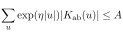
For the kernel rows, let Kab(u) be a cover coefficient with
Searchable transcription
X
u
exp(η|u|)|Kab(u)| ≤A
for each pair of finite residue types a,b. A routed term is its scalar multiple of adjoint transport along its designated walk, retained when length , and included only in the endpoint congruence class. Suppose length
 ). The full flat term is
 ) times the identity on color space, without the cutoff. Unitary adjoint action bounds the operator norm of each routed term

If link chords are h, a retained transport differs from the identity by at most 2 colorScale
 R h. For an omitted term the length inequality implies

Searchable transcription
ηR/D ≤η + η|u|,
1 ≤exp η · exp(η|u|) exp(−ηR/D).
Thus both kinds of difference are bounded by

Searchable transcription
J widen(R, h, η/D) exp(η|u|)|Kab(u)|,
J = 1 + 2 colorScale Cch + exp η.
Sum first on the cover. Each u contributes to exactly its endpoint congruence class; summing over endpoints therefore costs only the finite residue census, even on short tori with many windings. Absolute convergence allows the order of these nonnegative bounds to be interchanged. If there are  source types and
 target types, the convenient common row and column bound is

Searchable transcription
CK = (na + nb)AJ.
Both the cut nonlinear matrix and the full flat matrix have row and column sums at most and their difference has row and column sums at most
 widen(

For the same-level lanes, the ordered coordinate route to u has length |u| and . For the fine-to-coarse row, its route goes from a residue lift to Lu; its length is at most L|u|+4L. Both cases satisfy the preceding inequality with
 . The replica background has either identity links or original coarse links, so it preserves the required chord bound. Apply this calculation to the F, I and N rows with

Searchable transcription
A = max(max(0, E), E/L2), τ = η/(5L).
Take the maximum of 1 and the three corresponding values, and the common exponential-chart radius. This proves all the kernel-chart estimates used below, uniformly in the period and cutoff, with their row and transpose-row bounds. All constants are chosen after the block length L has been fixed.
Clean-hull guide comparison
The guide is the pair of coarse response fields Mv,Mw, while its linear comparison is obtained by applying the flat F and I rows to the linearized field ). There is also an N row. Its linear comparison vanishes identically: the supplied stationary identity is flatN
 = 0, and
 has precisely the coordinate form
 a. This includes harmonic coordinates; no scalar-mode deletion is used.
On a clean radius-B/4 hull agreeing with exp a, the clipped vision field equals the unclipped plotted field of exp a at every coordinate read by a guide row. The row’s reach is at most till(
 ); the plotted field needs only R+4 further sites, still within the same hull by the room inequalities. Cleanliness makes the retained indicator equal to one and makes the clipping factor min(1
 temp
 toll) equal to one. The row itself can also be replaced by its value at exp a by its local dependence on this hull.
Here is the resulting quantitative calculation. Suppose the nonlinear row Q has row bound X and differs from its flat row D by row bound XW. Suppose also

Searchable transcription
∥xlin(a)j∥≤Z, ∥plotted(exp a)j −xlin(a)j∥≤U.
Writing (exp
 = plotted(exp
 ), and
 ), the exact decomposition

Searchable transcription
Bf −Dg = B(f −g) + (B −D)g
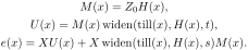
and the row-sum inequality give . All equalities before this bound are restricted to the same clean hull. In the source the uniform kernel-chart and plotted-chart estimates supply positive constants
 and
Searchable transcription
M(x) = Z0H(x),
U(x) = M(x) widen(till(x), H(x), t),
e(x) = XU(x) + X widen(till(x), H(x), s)M(x).
Here t is the lower-stage width divided by the positive block length. If H has rate 1/2 and is eventually nonnegative, broadening by widen preserves that rate: its bound is a radius factor times H plus an exponentially small cutoffterm. Products in the displayed formula therefore have rate
 1. The same e bounds the two guide differences and the nonlinear N guide itself, since its linear part is zero. The kernel-chart and plotted-field estimates of this chapter give these constants.
Stationary cancellation in every signed orientation
The stationary comparison uses a single supplied pair of quadratic beds and their common diagonal and roll identities. Their attached path realizations, positive floors, and invariance under signed coordinate changes are chosen together. Let W be the installed stationary map, U its extracted fine-field matrix for the chosen forest, and probe
 . The diagonal action identity reads

Searchable transcription
Kcoarse = UTKfineU + penalty · DT
0 D0.
For coarse logarithmic data a, the shifted fine field has color-coordinate vectors U a, while its residual has vectors a. Pairing this matrix identity with each color coordinate and summing gives

Searchable transcription
fineEnergy(shifteda) + penalty∥residual(a, shifteda)∥2
= coarseEnergy(a).
This is an identity of quadratic forms, including zero harmonic modes.
The same identity holds after any signed coordinate change. To justify the noise part, apply the exact signed covariance of the actual nonlinear predictor and noise energy to the exponentiated fields exp(t a), exp(t shifted a), divide by , and pass to their already established quadratic limits. The invariant fine and coarse bed metrics give the other two terms. Thus no isotropy of individual matrix entries is assumed.
Write w for the coarse linear moment field of the transformed input, u for the fine linear moment field of its transformed shifted field, and v for its linear noise field. The attached path realization and floor identify moment-square sums with the corresponding bed energies. The preceding energy identity is therefore

Searchable transcription
∥u∥2 + ∥v∥2 = ∥w∥2,
where the norms here are finite counting sums of squared color norms. Let F,I,N be the full flat rows, and put . The N row annihilates w. The diagonal roll and cross roll identities then give

Searchable transcription
w = F TU1 + ITV1, w = F Tu + ITv.
The transpose here means the adjoint for the counting inner products. Pairing the first equality with w gives

 . Pairing the second with w gives
 Expand squared differences and use these three equalities to obtain

Searchable transcription
∥U1 −u∥2 + ∥V1 −v∥2 = 0.
Every summand is nonnegative, so and
 at every row. This proves equality of linearCost and linearGuide in every signed orientation. Subtracting the linear copy then gives precisely the uncut spring cancellation used below.
Nearest group points and the analytic focus
All matrix norms in this paragraph are Frobenius norms, with the real inner product. Compactness of the closed unitary matrix group gives a nearest group element to every matrix X. Left or right multiplication by a group element preserves this minimization property, by unitary invariance of the norm.
If 1 is nearest to X, differentiate the squared distance exp(
 at its minimum
 for every Lie algebra matrix Y. The derivative is zero, so X
 1 is orthogonal to the Lie algebra. In general, if u is nearest to X, left multiplication by
 gives

Searchable transcription
u ∗X −1 ∈lie(G)⊥.
Here u* denotes the adjoint matrix of u. Consider the tubular map

Searchable transcription
T(a, n) = exp(colorMat(a))(1 + n), n ∈lie(G)⊥.
It is analytic and its derivative at (0,0) is colorMat( This is an isomorphism by the orthogonal tangent/normal decomposition. The inverse function theorem therefore gives a local analytic inverse near
 = 1. Define focus(
 ) as the exponential of the tangent coordinate of that inverse.
Every nearest point must agree with focus sufficiently near 1. To prove this without assuming continuity of a minimizing selection, choose any nearest ). Its minimizing property gives

 , hence
 . Thus
 1. Its normal coordinate

 1 tends to zero and is orthogonal to the Lie algebra by the preceding variational identity. Its tangent coordinate
 ) = log
 ) also tends to zero. Moreover
 exactly. Both coordinates therefore lie in the inverse-function neighborhood and equal its unique inverse coordinates, proving
 ) = focus(
 ). If there were exceptional nearest points arbitrarily near 1, choosing one at each exceptional X would contradict this conclusion. Thus every nearest point equals focus there.
This proves local uniqueness simultaneously over all components of the group. Translating X by a nearby group element extends the same uniqueness radius to a tube about the whole group. Differentiating the tubular inverse gives

Searchable transcription
D(mat ◦focus)(1) = orthogonalProjectionlie(G).
Indeed the inverse derivative sends colorMat( )+n to (a,n), and differentiating the exponential discards n. Analyticity makes this a strict derivative. Consequently, for every
 0, after shrinking the neighborhood of 1, nearest points u of X and v of Y satisfy

Searchable transcription
∥mat(u) −mat(v) −projectionlie(G)(X −Y )∥≤ε∥X −Y ∥.
These prove the focus properties used in the frame and predictor derivatives from the local group chart and the ordinary inverse function theorem.
Analyticity of the normalized frame
This is a fixed-period assertion; no volume-independent analytic radius is claimed here. Let v be the logarithmic input and its actual frame matrices at the patch points, with
 the distinguished center. At
 = 0 all path products equal 1. The identity frame minimizes the nonnegative frame score with score zero; uniqueness of the minimizer identifies the selected frame with it. The minimum branch has an open neighborhood of this input because its cutoffis positive. Continuity of the unique selected minimizer therefore gives continuity of all
 at zero. On that neighborhood all frame tags select this same frame.
The frame self-consistency condition says that is a nearest group element to
 ) = average
 average
 travel

This finite expression is analytic in v and the matrix array H: its path products are finite products of exponentials and adjoints. At ( 1), every cloud is 1. Continuity then puts every cloud in the neighborhood where its nearest group element equals the analytic focus map. Thus the actual frame solves the analytic equations

Searchable transcription
Fp(v, H) = Hp0 −1
if p = p0,
Fp(v, H) = Hp −focus(cloudp(v, H))otherwise.
Here focus is viewed in matrix coordinates. To apply the implicit function theorem, compute the derivative in the H variable at (0,1). If an array h belongs to its kernel, then = 0 and

Searchable transcription
hp = Aforp ̸= p0, A = projection(averageq hq).
Let N be the positive number of patch points. Averaging gives average . Since projection(
 , its defining equation yields
 , hence
 = 0 and
 = 0. The derivative is an injective endomorphism of a finite-dimensional matrix-array space, so it is invertible.
For precision, an analytic equation )) = 0 and a continuous solution
 ) with invertible H-derivative identify that solution with the analytic implicit branch: apply the inverse function theorem to (
 )). Continuity puts the given solution inside its local inverse domain, where uniqueness forces equality. This proves analyticity of the actual frame. It supplies the analytic frame input used in the following predictor calculation. The nearest-point, self-consistency and selected-minimizer arguments in this chapter establish the geometric properties used here.
First derivative of the actual rooted predictor
For coarse root y and patch points p,q, let fee ) be the tangent link sum along the actual ordered route from p to q in order o, embedded at y. Define

Searchable transcription
tapy(p; a) = −averageq averageo feey(p, q, o; a).
Each color coordinate of tap is the corresponding scalar path functional applied to the color-coordinate input. The derivative of a route product at the identity is colorMat of its link sum, by differentiating its finite product of exponentials; reversed links contribute with a minus sign. Let
 ) be the actual normalized frame matrix near zero, and let
 be its derivative in direction a. The local frame equation says that
 ) is the nearest-group focus of its averaged cloud. Differentiating that cloud gives average
 + colorMat(tap
 )). The derivative of focus at 1 is the orthogonal projection onto the matrix Lie algebra. Hence

Searchable transcription
dp = projection(averageq dq) + colorMat(tapy(p; a)).
The frame at the distinguished patch center is identically 1, so
 = 0. Subtracting its equation eliminates the common projected average:

Searchable transcription
dp = colorMat(tapy(p; a) −tapy(p0; a)).
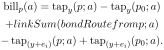
The local analytic frame equation and its normalization are the inputs to this differentiation; the subtraction shows explicitly why the derivative is independent of the frame tag. For a coarse bond (y,i), a connector consists of the left frame, the actual length-L bond route, and the inverse right frame. Its derivative is therefore colorMat of
Searchable transcription
billp(a) = tapy(p; a) −tapy(p0; a)
+linkSum(bondRoutefromp; a)
−tap(y+ei)(p; a) + tap(y+ei)(p0; a).
Near zero every connector is near 1. The best-predictor branch is open and is used at zero because its cost there is zero and its cutoffis positive. Thus the actual predictor near zero is the nearest-group focus of the weighted connector average, irrespective of its fallback tag. The connector average equals 1 at zero. It is analytic because the frame and finite route maps are analytic, and focus is analytic near 1; consequently the actual predictor is analytic near zero.

Searchable transcription
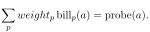
Differentiating the weighted average gives colorMat(P
p weightp billp(a)). This lies in the Lie
algebra, so the focus derivative leaves it unchanged. Expanding the definitions of tap, the rooted
path functionals, and the probe matrix shows coordinate by coordinate that
Searchable transcription
X
p
weightp billp(a) = probe(a).
The patch weights sum to one; this retains both frame-center subtraction terms. Thus the predictor equals 1 at zero and its literal first derivative is colorMat(probe( )), exactly the derivative used in the noise Taylor estimate. The remaining foundation of this calculation is the local analytic frame construction and focus derivative, rather than any limiting or averaged predictor.
Uniform predictor linearization and entry bounds
For a fixed patch and kernel, the predictor at one coarse bond reads a finite cover stencil. Include all vertices on every ordered route between patch points, the translated copy of this set at the other bond endpoint, and every straight length-L connector from a patch point. Call their union If two cover fields agree on links rooted in
 , every route product, axial frame, via-frame value and score agrees. Their minimizing frame also agrees by the supplied frame uniqueness; in the fallback branch their axial frame agrees directly. Thus their actual predictor values agree with the same endpoint tags and connector tag. Taking the maximum route distance of these finitely many roots defines predictionReach. Agreement on that parent-distance hull therefore suffices for predictor equality.
At fixed volume and fixed tags define

Searchable transcription
penalty · curvature(exp b · prediction(exp a, k)−1)
Zk(a, b) =
p
at the specified coarse bond. This is analytic near zero by the local analytic predictor theorem, matrix multiplication and adjoint, and the linear matrix formula for curvature. At zero the predictor is 1 and = 0. Its derivative is

Searchable transcription
zlin(a, b) =
p
penalty · (b −probe(a))
in the physical color coordinates: differentiate the predictor to obtain colorMat(probe( )), differentiate exp b, and use skew adjointness to differentiate the inverse. The curvature derivative recovers the difference. Taylor’s theorem gives a linear bound and a quadratic remainder. Since there are finitely many tags and bond positions on a fixed torus, a maximum of their constants and a positive minimum of their radii makes the bounds simultaneous there.
To remove volume dependence, choose one reference torus with coarse side 1 so large that every point of
 lifts uniquely from its fine torus. One explicit choice is
 + 2, where M is the largest absolute coordinate of a stencil point. For any input torus and any bond rooted at x, fill the reference fine logarithmic field by pulling back the actual input values under

Searchable transcription
y 7→wrapf(lift(y −embed(0))) + embed(x).
Fill its coarse logarithmic field constantly with the actual coarse value at the bond being read. Neither operation increases the supremum norm. Put the original left and right frame tags at 0 and  of the reference coarse torus; these sites are distinct because
 1. Put the original connector tag at the reference bond. All predictor stencil reads then agree exactly for every scalar multiple
 ), even if the original torus identifies different stencil points. Thus the nonlinear Z values agree
at = 1 and their linear terms agree by uniqueness of the derivative at
 = 0. The reference-torus Taylor bounds consequently give constants
 independent of the input volume and all its tags:

Searchable transcription
∥zlin(a, b)∥≤Cz max(∥a∥, ∥b∥),
∥Zk(a, b) −zlin(a, b)∥≤Cz max(∥a∥, ∥b∥)2
when the maximum is at most The local analytic predictor theorem and its derivative formula are the inputs to this Taylor argument; the transplantation adds no new branch choice.
The entry field is the direct sum of the fine plotted moment and Z. Its linear counterpart is the direct sum of and
 . For logarithmic inputs bounded by H, combine the plotted comparison already proved with the last inequality. If
 is its plotted constant, set

Searchable transcription
M = (Cx + Cz)H,
W = CxH widen(R, H, widthtop) + CzH2.
Then each linear entry has norm at most M and each entry-minus-linear-entry has norm at most W, simultaneously in the two kinds of row. For = till(
 ) and H of rate
 1/2 these have rates
 1/2 and
 1. The entry is gauge covariant by predictor covariance and curvature conjugation. It is local on the protected hull: the plotted component uses its cutoffstencil and the Z component uses predictionReach together with the coarse link at the row root. These establish the entry-near and entry-locality inputs used next.

Searchable transcription
For completeness, the full and cutofflinear rows have uniform stencil bounds at every cutoff,
not merely at till(x). A discrete curl has norm at most 4∥v∥. Summing a path row against its
weighted absolute coefficient budget gives ∥ellLine(v)∥≤4 paths∥v∥. Terms omitted beyond R
√
cost at most 4 paths∥v∥exp(−widthtopR). The direct-curvature term has bound 4
direct∥v∥; the
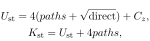
noise term has bound Cz∥v∥. Thus, writing
Searchable transcription
Ust = 4(paths +
√
direct) + Cz,
Kst = Ust + 4paths,
both full and cutoffrow norms are at most and their difference is at most
 exp(
 The cutoffbound follows by comparing to the full row and using exp(
 1. Absolute summability justifies every linear path sum and its subtraction.
These bounds also give the spatial impulse estimate used in the plate prices. If a single-link input of color a is at parent distance g from a row root, the cutoffrow at s is zero whenever  + predictionReach +4
 For
 predictionReach +5 choose
 predictionReach
 Compare both cutoffs R and s to the full row and apply their tail bounds; if R is too short the row is already zero. The result, also covering the nearby case by the uniform cutoffbound, is

Searchable transcription
exp(widthtopg)∥barFieldR(singlelinka)∥
≤2Kst exp(widthtop(predictionReach +6))∥a∥.
From a shell comparison to the tree-slice link estimate
For a differentiable group-valued curve ) with
 (0) = 1 and matrix derivative colorMat(
 ), the norm of its difference quotient gives

Searchable transcription
chord(U(t))/|t| →∥a∥ast →0, t ̸= 0.
Source: A Wilson Yang–Mills Construction: A Natural-Language Mathematical Exposition. Both papers belong to one Zenodo record. No external funding.