Local nonlinear geometry and estimates · Part 7

The short correction family

The short corrections and Gaussian chains are organized so that locality can be priced before the full connected expansion is summed. A chain letter remembers its genuine path support and itinerary; changing to a smaller nominal support would invalidate the later hit counts. The inverse and logarithm series are absolutely convergent under the displayed smallness conditions, so their pointwise exponent identities may subsequently be integrated.

Budget language as inequalities The correction families are organized by the upper bounds they spend and the positive estimates that absorb those bounds. A price is an explicit coefficient in such an inequality; income is a proved lower estimate; and a payment is the displayed domination after the parameters have been chosen in the permitted order. These terms do not describe a new probability law. Retaining their weights and exponents is essential because the same finite store must absorb the fine, noise and coarse contributions simultaneously.

The local short letters have three kinds. At a signed row root o outside the 200B seed neighborhood, the energy letter is

Searchable transcription

−βorientation · [enforce(2a)(u, booth(o)) · light(u)
+extracted(μ)].

It is zero inside that neighborhood. The second letter is the local condensation term, set to zero when either endpoint of its fine bond touches the 200B seed dome. The third is the cut-off Haar logarithm gentry, retained only at hot links outside the plaza of the 304B seed dome. Their geometric sleeves are fixed neighborhoods of their row or bond captions.

On the original seeded sector the light term equals the original energy debit at a remote row. The noise row equality is definitional. For the curvature row, turn the actual fields, tags and seed store together; the seeded sector and positive likelihood give the local Interior bounds. If the soft retention threshold at a possible curvature read is below 2, the room inequality places that read in this interior and its plaquette toll is at most. If the threshold is at least 2, the universal chord bound supplies retention. Thus the retained high-stage path field is unchanged there, and the exact split-curvature identity identifies light with debit. This reasoning uses actual sector membership only for this equality, not for the all-field bounds below. Let) be the protected-mean path envelope already proved, of rate1. The extracted term is a sum of at most two nonnegative half-squares of parent path values. At a remote row its absolute value is therefore at most 2(

Take from “Light estimates on the annulus,” with grafted tangent bound 4 fiery(). The soft-square and mismatch estimates there have rate2, and the two quartic or squared-guide corrections have rate2; weakening the latter gives rate2. Take = dim g pulseHead(repair) from the preceding local plate comparison. Its repair envelope has rate2, its window census has rate zero, and its fixed inverse-window constants do not depend on has rate2. These are the actual two bounds needed here. The Haar estimate gives gentry fiery. To use the light estimate for arbitrary input, split according to whether its enforcement profile is zero. If it is nonzero, its protection property bounds every tangent value read by the booth by 4 fiery. The distant-field identity then supplies precisely the grafted condition on the common clean radius- hull. The profile is at most one, so its product with light is bounded by. Outside the 200 exclusion all these hull and parent-path conditions follow from the same seed separation. For 02 betaF and 01, the energy letter is bounded by

Searchable transcription

Wshort(x) = 2betaF(x)[J(x) + A(x)2].

Its rate is1/2: betaF has rate 1, J has rate3/2, and has rate2. The condensation and Haar letters have bounds and Cfiery of rate1/2 as well. Thus their sum

Searchable transcription

Eshort = Econd + C · fiery +Wshort

is a common eventually nonnegative envelope of rate1/2 for all three kinds, all fields and all admissible. A bond whose endpoints touch a dome has its parent in the one-site enlargement; conversely a bond not touching it has its parent outside it. These elementary endpoint facts justify the condensation exclusion used here. The light-remainder, remote-condensation and grafted-signal estimates of this chapter establish the three inputs to this assembly, together with the mean and Haar bounds.

A fixed multiple of the small-field scale for the base stroke

Searchable transcription

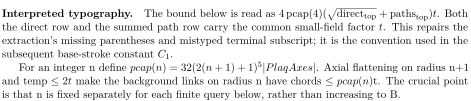
pdirecttop + pathstop)t. Both
Interpreted typography.
The bound below is read as 4 pcap(4)(
the direct row and the summed path row carry the common small-field factor t. This repairs the
extraction’s missing parentheses and mistyped terminal subscript; it is the convention used in the
subsequent base-stroke constant C1.
For an integer n define pcap(n) = 32(2(n + 1) + 1)5|PlaqAxes|. Axial flattening on radius n+1
and temp ≤2t make the background links on radius n have chords ≤pcap(n)t. The crucial point
is that n is fixed separately for each finite query below, rather than increasing to B.

First consider any fine plaquette of replica( ) with a clean radius-five hull about its coarse parent. Use = 4. Replica links in that hull are either identity or a coarse link in the chosen gauge, and hence have chordspcap(4). Replace links outside the hull by 1. Its plaquette product is unchanged, so its chord is at most 4 pcap(4)t. The same bound applies to its curvature norm.

For the fine base moment row, every retained path slot ends at a plaquette whose parent has a clean radius-five hull inside the original radius-B clean region. Its actual path length is bounded by till(), and the room inequalities ensure this inclusion. Its adjoint transport preserves curvature norm. Summing against the absolute path coefficient budget, and including the direct curvature coordinate, therefore gives

Searchable transcription

∥XfR(replica(V ))∥
≤4 pcap(4)(
q
directtop + pathstop)t =: C1t.

No single gauge is needed for every slot: only its curvature norm is estimated.

For the noise base stroke, instead fix = predictionReach(). Flatten on that fixed hull and extend its logarithm to a global bounded field b with). Its linear copy a has norm at mostand exponentiates exactly to replica(exp b). Predictor locality identifies the actual base noise stroke in this gauge with zTest(), with its original tags. Its uniform Taylor estimate gives

Searchable transcription

∥zTest(a, b)∥≤J∥(a, b)∥2 + J∥(a, b)∥≤2JAt

eventually, since1 and the chart radius. Gauge covariance transfers the bound back. Thus is one positive constant bounding every clean-hull base stroke by that constant times t. This proves the crowns input to the global mean bound without spending an extra growing-radius factor.

Global mean and stationary residual

The global mean bound uses selected rows, the frozen cutofffield, and the inverse-window bounds; it is separate from the sharper remote path estimate. Let the clean-background base stroke be bounded by, every guide by Mt, the oriented cutoffoperator by N, and the saved field by 2Kt, where K is the fixed shell width. On a selected row, seed separation supplies the clean hull needed for the base-stroke estimate. At zero hot input,

Searchable transcription

∥priced(0)∥≤scale[A0 + M + 2NγK]t =: b1t.

An unselected row is zero and satisfies the same bound. This uses the saved-field bound globally, without requiring a common global gauge.

The linear bill is the transpose form applied to priced(0). Its row-sum bound Y gives . Let P be the inverse-column pad and. Its column bound gives. Summing its color-coordinate bounds yieldsdim(

The stationary residual has a useful exact form. Symmetry of gives

Searchable transcription

Aμcount + b = −A(P −A−1)Tb.

The pad discrepancy and plate row bound Q therefore imply

Searchable transcription

|Aμcount + bi| ≤Q distPay(B)b0t.

Choose = 1 + max( dim( It simultaneously bounds priced(0), the linear bill and the mean by t. The residual envelope above has any prescribed rate k: scraps(), and hence distPay(), has rate k+1/2, while t has rate1/2. This supplies the mean/residual hypotheses of the correction budgets. The clean base-stroke and uniform maximum estimates proved here give and M.

Exact Gaussian exponent rearrangement

Let D be the form matrix, the dormant diagonal, the count-coordinate mean, b the linear bill, and the positive reference covariance. The lifted tangent input is with. The affine-square sum has the exact polarization identity

Searchable transcription

liftSq(μ + gz) = liftSq(μ)
+g⟨z, b + DTDμ⟩+ g2⟨z, DTDz⟩/2.

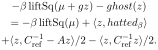
This follows by expanding each squared affine row and summing the finite color coordinates. The dormant mean vanishes, so2. Using = 1 and gives

Searchable transcription

−β liftSq(μ + gz) −ghost(z)
= −β liftSq(μ) + ⟨z, hattedβ⟩
+⟨z, C−1
ref −Az⟩/2 −⟨z, C−1
ref z⟩/2.

The last term is the reference Gaussian exponent. The preceding quadratic term is the correction expanded by the itinerary chain; the linear term is the first correction. The inserted ghost supplies exactly the dormant diagonal needed to complete A, and its normalized dormant Gaussian integral is one as shown earlier. This equality is pointwise algebra and remains valid where a later profile vanishes; it assumes no sector event.

Pointwise Gaussian chain corrections

Write A for the completed plate, for the symmetric reference covariance, and for its small discrepancy. The linear correction vector is

Searchable transcription

hattedβ = −gStep(β)−1(Adrift + b).

Searchable transcription

For each fine link e its scalar correction is P
c olor z(e,j) hatted(e,j). Multiply this by aperture(e),
the cone profile at twice the chosen enforcement radius on hot links and the value 1 on other links,
to obtain qfirst.
For an itinerary of n+2 link steps, the quadratic correction is half the bilinear pairing between
its starting and ending z vectors with the ordered matrix-block product

Searchable transcription

−Serr · · · −SerrA,

containing n+1 discrepancy factors and one terminal A. Multiply it by the two endpoint apertures to obtain chain. Summing itineraries at fixed starting link and n restores exactly the matrix product ( in that quadratic form: the intermediate link and color sums are precisely matrix multiplication. The terminal A is retained in both the formula and its price.

Dormant plate rows are identity rows and the reference covariance has the same identity completion. Therefore has zero entries whenever either endpoint is dormant. The linear bill and mean vanish there too, so hatted is zero at dormant coordinates. A nonzero quadratic chain consequently has hot starting and ending links: every nonzero discrepancy factor forces hot endpoints, and the final A cannot join a hot link to a distinct dormant identity row. Induction over its discrepancy factors proves this for every n. Let t and = gStep( 0. At a hot endpoint where its aperture is nonzero, the cone bounds t. The triangle inequality gives

Searchable transcription

∥atmos(z)e∥≤g−1t(4a + K) = heat(a, K, t, β).

Thus an envelope bounds every endpoint color coordinate. The aperture is at most one. If hatted, the finite color sum yields

Searchable transcription

|qfirste| ≤dim(Color)UM.

This holds at dormant links as well because their linear correction vanishes. For the chain, put = dim( = distPay(), and. The discrepancy has entry bound, whereas the terminal plate has entry bound Q. Summing its n+1 intermediate color indices bounds each entry of the prescribed block product by

Searchable transcription

Rn+2
c
QMn+1
err .

The convenient extra color factor is included in the source’s product estimate. The two endpoint color sums therefore bound the half-bilinear form by

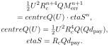
Searchable transcription

1
2U2Rn+4
c
QMn+1
err
= centreQ(U) · etaSn,
centreQ(U) = 1
2U2R4
cQ(Qdpay),
etaS = RcQdpay.

A nonzero term must also be armed: every itinerary hop has parent distance at most 3B. Otherwise its corresponding discrepancy or plate block vanishes by the finite-range estimates. Define capQ to equal the displayed center-times-ratio power on armed itineraries and zero on the others. Splitting into zero aperture, zero bilinear form, and nonzero cases proves pointwise for every z. This explains why these optional terms use endpoint cutoffbounds rather than a separate Gaussian tail event.

Convergent inverse and logarithm expansions

Searchable transcription

Weighted absolute row and column prices multiply under matrix multiplication. If a matrix E
has price q < 1 at a nonnegative width, En has price qn, so its entries form absolutely convergent
geometric series. The finite identity P
n<N En(I−E) = I−EN and EN →0 give P En = (I−E)−1,
proving invertibility at the same time.
There are two different orders of multiplication needed here. If AP −I = E, then

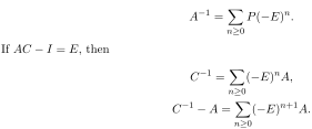
Searchable transcription

A−1 =
X
n≥0
P(−E)n.
If AC −I = E, then
C−1 =
X
n≥0
(−E)nA,
C−1 −A =
X
n≥0
(−E)n+1A.

These follow by multiplying the geometric inverse of I+E on the appropriate side. The order is essential because the matrices need not commute. Absolute entry convergence permits the fixed matrix multiplications and the removal of the zeroth term. For a real matrix A whose interpolation) remains invertible on [0,1], the elementary determinant derivative gives

Searchable transcription

d/ds log | det Gs| = trace((A −I)G−1
s ).

Searchable transcription

To derive it at s = r, factor Gs = [I +(s−r)(A−I)G−1
r ]Gr. The coefficient of t in det(I +tB) is
trace B, as follows directly from the determinant polynomial. Differentiate the factored determinant
and then log|·|. The inverse is continuous along this compact interpolation by the adjugate formula
and nonvanishing determinant. Integrating therefore gives

Searchable transcription

log | det A| =
Z 1
0
trace((A −I)G−1
s )ds.

For the positive plates used here det 0, so this is log det Let be its inverse-column pad and. The uniform discrepancy price scraps( 1 gives

Searchable transcription

(A −I)G−1
s
=
X
n≥0
(A −I)Ps(−Es)n.

Searchable transcription

The pad Ps occurs once in each term; only the residual −Es is raised to the power n. This follows
from GsPs = I + Es, hence G−1
s
= Ps(I + Es)−1.
Each diagonal summand is continuous in s and bounded in absolute value by (Q + 1)payE · ρn.
The geometric bound is summable independently of s. Hence its interval integrals may be summed:

the sum of their integral norms is bounded by the same geometric series on an interval of length one. Write) for these diagonal integrals and localBase = lact(0). We obtain

Searchable transcription

log det A =
X
i
localBasei +
X
X
n≥0
lacti(n + 1).
i

Searchable transcription

Thus the local principal-window diagnostic is only the zeroth term; the remaining determinant
arms restore the full inverse exactly.
For any discrepancy E of price q < 1, apply the same argument to I+sE and expand its inverse
as P
n(−sE)n. The integrands E(−sE)n have uniform bound qn+1, giving

Searchable transcription

Z 1
log | det(I + E)| =
X
X
0
[E(−sE)n](i,i)ds.
n≥0
i

In particular yields. Both A and have positive determinants, so the right side equals log det + log det. These source-arm terms therefore represent the actual covariance normalization defect. All exchanges here use uniform summable entry bounds, followed by finite coordinate sums; no volume factor is treated as a local price.

Itinerary receipts and scalar arm identities

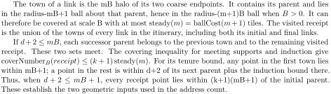
An itinerary of k hops is a list of k successor fine links, with the initial link retained separately. A hop is armed at radius d when some coarse endpoint of the first link is within d of some coarse endpoint of the next. Each parent is within one site of either endpoint, so an armed hop moves parents by at most d+2.

Searchable transcription

The town of a link is the mB halo of its two coarse endpoints. It contains its parent and lies
in the radius-mB+1 ball about that parent, hence in the radius-(m+1)B ball when B > 0. It can
therefore be covered at scale B with at most steady(m) = ballCost(m+1) tiles. The visited receipt
is the union of the towns of every link in the itinerary, including both its initial and final links.
If d + 2 ≤mB, each successor parent belongs to the previous town and to the remaining visited
receipt. These two sets meet. The covering inequality for meeting supports and induction give
coverNumberB(receipt) ≤(k + 1) steady(m). For its tenure bound, any point in the first town lies
within mB+1; a point in the rest is within d+2 of its next parent plus the induction bound there.
Thus, when d + 2 ≤mB + 1, every receipt point lies within (k+1)(mB+1) of the initial parent.
These establish the two geometric inputs used in the address count.

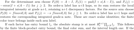
For a sequence of matrices and a fixed itinerary, multiply their color blocks in its link order. Keep only itineraries returning to their initial link, take the color trace of that block product, and integrate s from 0 to 1. Call this scalar its stamp. Expanding matrix multiplication shows that summing stamps over all k-hop itineraries restores the integrated diagonal trace of 1). There are finitely many itineraries at fixed k; continuity of the matrix factors gives integrability and permits interchanging these finite sums and the integral.

Searchable transcription

For the determinant arm choose Ps(0) = A −I, Ps(1) = pad(I + s(A −I)), and Ps(j) =
−error(I + s(A −I)) for j ≥2. Its order-n label has n+3 hops, so its sum restores the local
integrated intensity at grade n+1, retaining n+1 discrepancy factors. For the source arm choose
Ps(0) = flawed(A) and Ps(j) = −s flawed(A) for j ≥1. Its order-n label has n+1 hops and
restores the corresponding integrated grade-n note. These are exact scalar identities; the finite
color trace belongs inside each arm label.
Q
If each factor has entry bound lj, the absolute stamp is at most Rk+1
j<k lj. This follows
c
by the finite block-product entry bound, the final color sum, and the interval length one. If the

itinerary is not armed at the common factor range, one factor block is zero, so its stamp is zero. This proves the arm representations and the pointwise pricing mechanism used above.

Counting all itinerary addresses

Both the chain coefficient bound and the The order- itinerary price is route/support price arise at every step. The extraction’s unparenthesized is interpreted accordingly, consistently with the repeated chain estimate later in the same construction.

An order-n ledger with u extra steps consists of a starting fine link and an itinerary of n+u hops. Its receipt is the prescribed union of enlarged neighborhoods visited along that itinerary. Put density( and abundance() = ballCost( + 2) density(). From any starting link an armed hop of radius d has at most abundance() possible next links: every such link has parent in the radius-d+2 neighborhood, and the fine-link caption census has density(). Induction over the hops therefore bounds the number of armed k-hop itineraries by abundance(

The receipt geometry gives two bounds when and 0. Its B-covering number is at most (k+1)steady(), and if a fixed site x belongs to its receipt, its starting link has parent within distance (k+1)(mB+1) of x. The underlying definitions of visited receipts give these covering and tenure bounds; they remain the immediate geometric inputs here. Their effect on the count is as follows. For coefficients 0 on armed addresses and zero elsewhere, the tariffat order n includes exp(2) and exp( coverNumber). Bound the latter by exp( 1) steady()). The number of eligible starting links is at most

Searchable transcription

ballCost((n + u + 1)(mB + 1)) density(L).

The elementary inequality and the four-dimensional ball formula give

Searchable transcription

ballCost((n + u + 1)g) ≤ballCost((u + 1)g)16n.

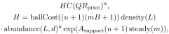
Multiplying this starting-link count, the armed-hop count, and the coefficient/tariffbounds yields, at each x, an order-n total at most

Searchable transcription

HC(QRprice)n,
H = ballCost((u + 1)(mB + 1)) density(L)
· abundance(L, d)u exp(Asupport(u + 1) steady(m)),

= 16 abundance() exp( steady(

When Q2, its sum over n is at most 2HC. All terms are nonnegative. To pass from the finite order-n sums to the countable ledger sum, first bound every finite subset within its finitely many order fibers, then apply the convergent geometric bound. This proves the asserted sales inequality and its summability, retaining every address even when different itineraries revisit the same link.

Pointwise determinant and source arm prices

For the determinant arm the ordered factors along its n+3 hops have respective entry prices Q+1, payE, and n+1 copies of scraps(). Each factor has range at most 3B: the plate term uses its B/2 stencil, the inverse-column pad its window, and its discrepancy the enlarged window stencil. The

common interpolating parameter 1] preserves these bounds and their positive floors. The product entry estimate, followed by the color trace and s integral, gives

Searchable transcription

|ArmA(n,e,p)| ≤Rn+4
c
(Q + 1)payE · scraps(B)n+1
= centreA · etaAn

Searchable transcription

on armed itineraries, and zero otherwise. Here centreA = R4
c(Q + 1)payE · scraps(B), etaA =
Rc · scraps(B), and Rc is the color dimension.
For the source arm all n+1 factors have entry price Q·distPay(B); the factors beyond the first
also contain the scalar interpolation multiplier, whose absolute value is at most one. Their range
remains 3B. Thus

Searchable transcription

|ArmS(n,e,p)| ≤Rn+2
c
(Q distPay(B))n+1
= centreS · etaSn

Searchable transcription

with centreS = R2
cQ distPay(B) and etaS = Rc Q distPay(B). These bounds are the actual
scalar arm prices before exponential expansion. They use the ordered-product and trace-integral
representation of the arms given in the itinerary section; the pointwise estimate sums their finite
internal color indices and integrates over an interval of length one.

From itinerary envelopes to support budgets

The general itinerary bound takes an armed-path coefficient of the form, supported on its predetermined receipt of halo4 and fixed number u of extra steps. Let abundance( bound the number of possible next links in an armed hop. Both this abundance and the fixed-step prefactor) have rate zero. The geometric receipt estimate gives the sales bound

Searchable transcription

2expoHead · Y

Searchable transcription

as soon as

Searchable transcription

16 abundance(L, 3B) exp(Asupport · steady(i) + 2ε)κ ≤1/2.

If has any negative rate, that condition holds eventually; multiplying it by the rate-zero abundance does not change its decay. Thus an envelope Y of rate b yields a sales bound of rate b. This numerical deduction is uniform in geometry; the itinerary address count and halo-cover estimate supply the quantities expoHead and steady used here.

Apply it to the determinant and source arms separately. The determinant arm uses center scraps() and ratio scraps(). The source arm uses = 1, center distPay() and ratio QdistPay(). All centers and ratios have every prescribed negative rate, so their sales budgets can have any prescribed rate b. Their pointwise bounds retain one scalar per actual arm, rather than splitting a trace into independently labeled colors. Applying the same bounds to the blank geometry supplies its determinant arm independently. The pointwise arm identities and the geometric itinerary estimate are still the inputs to this budget calculation.

Numerical budgets for the Gaussian chain letters

The mean/residual hypotheses are retained separately. They assert and drift + ), together with the shell access bound. For the physical beta band 02 betaF put