Quadratic kernels and their ultraviolet limit

Quadratic kernels and their ultraviolet limit

The quadratic analysis constructs the linear response around the flat configuration. There are three separate issues. The evaluated quadratic form on link potentials must converge; its curvature representation must remain positive and exponentially local; and the stationary predictor must have a regular Fourier symbol at the apparent zero-momentum singularity. The auxiliary metric amendment changes only directions not detected by curls. Thus retaining the physical potential precision is a proved identity, not an inference from positivity.

Flat quadratic ultraviolet convergence

Reading the finite linear records This opening convergence argument states the estimates required from a finite linear history before constructing that history below. A history, also called a horizon in the source notation, is a finite sequence of metrics and adjacent stationary response maps ending at the fixed bare quadratic form. Its price table records analytic widths, lower coercivity bounds and upper kernel bounds at each stage. A smoothing train is the finite chain of averaging patches defined in Section 5.8; a transition tower is the collection of auxiliary rows used to realize one adjacent response and its Gram identities. These names describe finite numerical and operator records. The later metric, tower and pinning calculations construct their required identities, so the opening conditional estimate is not an extra assumption of the public theorem.

Write for the positive lattice spacing at level i, with tending to zero. For a reporting level k put

Searchable transcription

T(k, i) = 2 + Z(k) + |ti −tk|,

where Z is nonnegative. Let denote the cover kernel of the quadratic action at level i constructed with finer cutoffn. The convention is the action Hessian convention; there is no additional factor one half. The kernel is obtained from the curvature kernel by composition on both sides with the lattice coboundary, so it describes the quadratic form on link potentials. It does not determine an arbitrary extension of the curvature metric away from curls. For0, let) be the weighted row bound of a cover kernel: for every output link and each fixed input orientation, sum the absolute kernel entries over input sites with weight then take the supremum over the output link and input orientation. This is the source’s RowCost at side one. Exponential weights control spatial locality as well as absolute summability.

A finite quadratic history has, at each, five real Laurent rows: an unamended two-form metric, its inverse, an amended metric, its inverse, and a residual Gram root Their weighted coefficient bounds have width 0 and price Ω()). At every torus period,

Searchable transcription

HH−1 = MM−1 = I,
F ∗F + cI = M,
Md1 = Hd1,
M(0) = I.

Searchable transcription

Here c > 0 is the direct clip coefficient; the full Gram factor is the stack (√c I, F). Both metrics
are symmetric with quadratic forms between η(J(i))I and Ω(J(i))I, where η > 0. The terminal
unamended metric is I. Each transition has a fine potential response A0, curvature response T, and
mixed, normal and image rows satisfying the stationary and Gram identities derived below. The
mixed row has bound Ω/L2; the normal and image rows have bound Ω. A word of r carried fine
differences of A0 or T has bound ΩL−1−r or ΩL−2−r, respectively, through order J(i + 1) −2. A

carried difference increments the fine residue, shifts the coarse displacement when that increment crosses its centered seam, and subtracts the original entry. Thus it is the actual fine difference, including the carry. These all-period conditions are constructed by the metric, positive-margin, auxiliary-tower and pinning arguments below; they are not additional assumptions of the public theorem. Put)). The spacing hypotheses are

Searchable transcription

0 < w(j) ≤min{1, P.α(j)},
yi ≤min{1, P.α(J(i + 1)), P.α(J(i))}
(i ≥e),

one-step price atblock( block(

Searchable transcription

P.Ω(J(i)) ≤B T(k, i)l
(k arbitrary, i ≥e),

for0 and a nonnegative integer. Here andΩare the width and upper-bound columns of the fixed price table. Each earlier history also uses the specified destination response , the compatibility condition called Flat.meshed in the source. Under these hypotheses there exist0, an integer0, and 0 such that, for all k and

Searchable transcription

Ryi(Qn,i −QN,i)
(1)
≤AT(k, i)d(aN/ai)c.

The source proves this through curvature packets. At the terminal comparison level N subtract the two saddle curvature kernels. Their strip bounds give a packet whose cost is at most

Searchable transcription

topTab(N) = 2|Faces|P.Ω(J(N)).

This packet represents the difference of the quadratic forms on every scheduled torus. Propagate it backwards from i+1 to i using the two histories’ fine response maps. The exact crossing identity preserves its representation of the quadratic difference; neutrality and translation covariance are retained. The weighted packet cost is multiplied by quote(). The width-crossing hypothesis licenses this propagation at width. In particular, this is an identity for the two actual histories rather than a comparison with a separately chosen limiting history. If is the propagated cost, the recursive majorization is

Searchable transcription

CN = topTab(N), Ci ≤block(i)−θCi+1.

One may first define a nonnegative majorant using the reciprocal recursive weight, called Stair.weight in the source. Its recurrence is exact before the one-step factor is replaced by its upper bound. Applying the polynomial-age decay lemma of Section 5.2 gives

Searchable transcription

Ci ≤AT(k, i)d(aN/ai)c.

Searchable transcription

In this particular terminal-only recurrence the majorant can also be written without the auxil-
iary weight notation. With tj = log(a−1
j ), it is

Searchable transcription

N−1
Y
bCi = topTab(N)
j=i
L−θ
j
= topTab(N)e−θ(tN−ti).

The empty product gives its terminal value, and each backward step has exactly the required contraction. Set0. The triangle inequality gives, whereas 2. The polynomial cap on the terminal price therefore gives

Searchable transcription

bCi ≤CT(k, i)l(1 + u)le−θu ≤C′T(k, i)le−θu/2.

The last constant is finite because the continuous function (1 + is bounded on [0 Since , this is the asserted estimate with2. The more general recurrence lemma below also allows forcing at intermediate levels. Neither argument assumes continuum convergence.

To recover the cover quadratic kernel, let be the lattice coboundary and set with interpreted as its two-point kernel. Finite support of gives a width-one row and column bound0 for this paragraph. Weighted convolution and the distance triangle inequality give

Searchable transcription

Rs(W(K)) ≤|Faces|2L2C

whenever the packet has width1 and cost C. This constant is independent of the torus size.

The required uniqueness concerns periodization of absolutely summable cover kernels, not inversion of a finite matrix. In the source these operations are respectively named Flat.resolve and FreeResolvent.resolve. Suppose two summable cover kernels give the same matrices on tori whose side lengths tend to infinity. For a fixed pair of cover sites, express a periodized entry as the sum over sites with the same torus image. For each fixed summand, eventual injectivity of wrapping makes its indicator tend to the indicator of the selected cover site. The absolute kernel entries form a summable dominating family. Dominated convergence recovers that cover entry from the torus entries. Both kernels have the same limit and therefore agree entry by entry.

Apply this argument to and). Their finite-torus quadratic matrices agree by the propagated packet identity, and both have summable rows. Thus their cover kernels agree. The preceding convolution bound proves (1), absorbingFaces into A.

For each fixed, (1) makes every entry of a Cauchy sequence, since tends to zero and 0. Let be its entrywise limit. Fatou’s lemma for the nonnegative weighted absolute entries gives

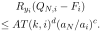
Searchable transcription

Ryi(QN,i −Fi)
≤AT(k, i)d(aN/ai)c.

The horizon strip bound and the polynomial cap on the upper-bound columnΩsimilarly give

Searchable transcription

Ryi(Fi) ≤B′T(k, i)l.

The limits obtained with different reporting levels k coincide by uniqueness of entrywise limits. Consequently one family works for every k. On levels before e it can be defined as zero because the conclusion imposes no requirement there.

Polynomial majorants and decay

Let be increasing scale times, with ∆log 3, and put, where 0. Then2 and. Suppose

Searchable transcription

fi ≤e−θ∆ifi+1 + gi
(i < N),
fN ≤gN,
0 ≤gi ≤Aτ d
i ,

with, and 0, uniformly in the schedules and terminal indices. Define

Searchable transcription

K = 2(d + 1)
θ
,
q = e−(θ/2) log 3 ∈(0, 1),
B =
A
1 −q.
Since K + τi ≥K, the inequality 1 + u ≤eu gives

Searchable transcription

K + τi+1 ≤(K + τi)e∆i/K.

Searchable transcription

Thus d/K ≤θ/2 implies

Searchable transcription

e−θ∆i(K + τi+1)d ≤e−(θ/2)∆i(K + τi)d ≤q(K + τi)d.

Backward induction proves, use. At an earlier index,

Searchable transcription

fi ≤(Bq + A)(K + τi)d = B(K + τi)d.

Searchable transcription

Finally K + τi ≤(K + 1)τi, so fi ≤B(K + 1)dτ d
i . This includes d = 0 and A = 0.

Searchable transcription

For the decaying version, suppose giec(tN−ti) has a uniform nonnegative polynomial majorant,
with c > 0. Put μ = min(c, θ/2) > 0, and multiply the recurrence by eμ(tN−ti). The new unknown
has contraction exponent θ −μ > 0; its forcing is polynomially bounded because μ ≤c. The
preceding induction gives
fi ≤A′τ d′
i e−μ(tN−ti)

for uniform. For the lattice schedule . A forcing supported only at automatically satisfies the weighted hypothesis, because its exponential factor is one on its support. This proves the decay estimate used in the flat overlap construction. The same argument extends to a well-founded collection of grades. At a grade j, permit polynomial forcing in finitely many strictly earlier grades, at the current and next scale. Sums, products, and integer powers preserve polynomial bounds. Next-scale ages are polynomially controlled when the block lengths are polynomially bounded in the current age, because + log(block( block(). Induction on the grade therefore supplies the forcing bound needed for the scalar recursion. For differences, include the absolute bounds from both histories, including the current grade, in the forcing polynomial; permit difference bounds only at strictly earlier grades. A finite sum of exponentially decaying polynomial bounds retains such a bound with the minimum positive exponent, and multiplication by polynomial absolute bounds preserves it. The scalar weighted recursion then closes the induction. This recurrence is applied to the one-step estimates for the actual histories constructed in the nonlinear and history-convergence chapters.

Independence of the evaluated quadratic kernel

Which quadratic object is independent The object compared here is the evaluated quadratic form on link potentials. The auxiliary two-form metric can change on directions not tested by the curl without changing that form. The word “shadow” in this particular calculation names the displayed modification of clip parameters in a second finite linear history. It does not introduce a source–readout framework into this companion paper. Equality is proved by the stationary matrix identities and backward induction from the common terminal form; no equality of the full nonlinear actions is inferred from it.

The horizon’s terminal quadratic form is the same fixed bare quadratic form for every admissible horizon. Its one-step stationary action identity is, on each finite torus,

Searchable transcription

Qcoarse = T TQfineT + b(I −probe T)T(I −probe T),

where 0 is the blocking penalty and T is the extracted stationary response. Here is the exact comparison algebra. Write P for the common probe, Q,R for two symmetric fine precisions, A,B for their symmetric coarse precisions, and T,W for the responses. The primal and dual equations are

Searchable transcription

QT = P TA, RW = P TB, A = b(I −PT), B = b(I −PW).

Taking the transpose of gives. Consequently

Searchable transcription

W T(R −Q)T = BPT −(PW)TA
= B(I −A/b) −(I −B/b)A = B −A.

The mixed terms cancel in their displayed order; no commutation of A and B is required. Thus equality of the fine quadratic forms implies equality of the coarse forms even if the auxiliary factorizations differ. Backward induction from the common terminal form gives equality at every level

on every scheduled torus. The periodization uniqueness argument above then gives equality of the summable cover kernels. This proves the quadratic-history comparison. The harmonic and scaled-exterior sections construct the responses and derive their primal and dual equations.

The comparison construction replaces each clip’s two numerical factors by) and with 0, retaining the relaxation, radius and slow selector. It retains the schedule, patches, smoothing indices and blocking penalty used by the block operator. The same terminal and backward comparison therefore applies to the original and modified horizons. Their evaluated quadratic cover kernels agree at every finite cutoff. This concerns the quadratic action on link potentials and does not identify higher-order horizon data.

Here is the entrance argument, called entrance_gate in the source. First choose the retained-support linear construction for the fixed kernel choice; it supplies a positive clip curve and a length demand Apply the linear horizon construction to the numerical schedule with its rearranged clip profile. For its price choice, set) = maxtickets(. The condition block() pays both demands, including auxiliary steps before the admitting tail. The delay at supplies the spacing hypotheses proved next. Apply the flat convergence estimate to the modified horizon to obtain one family, its polynomial absolute bound and its decaying difference bound. The exact comparison just proved, called same_shadow, identifies every original finite-cutoff quadratic output with its modified output. Equality of those sequences transfers their limits and difference bounds to every admissible original horizon. This proves the entrance statement once the retained-support construction is supplied.

Choosing the widths before the block lengths

For the fixed price table, choose) = min 0. Let) be the allotted bound for adjacent smoothing indices, and put

Searchable transcription

B(j, u) = |Faces|2[2/w(j)]h(j, u)2,
EP (j) =
l
2/w(j) + B(j, j)2 + B(j, j −1)2m
.

Searchable transcription

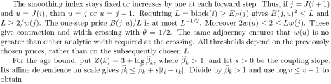
The smoothing index stays fixed or increases by one at each forward step. Thus, if j = J(i + 1)
and u = J(i), then u = j or u = j −1. Requiring L = block(i) ≥EP (j) gives B(j, u)2 ≤L and
L ≥2/w(j). The one-step price B(j, u)/L is at most L−1/2. Moreover 2w(u) ≤2 ≤Lw(j). These
give contraction and width crossing with θ = 1/2. The same adjacency ensures that w(u) is no
greater than either analytic width required at the crossing. All thresholds depend on the previously
chosen prices, rather than on the subsequently chosen L.
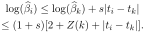
For the age bound, put Z(k) = 3 + log bβk, where bβk > 1, and let s > 0 be the coupling slope.
Its affine dependence on scale gives bβi ≤bβk + s|ti −tk|. Divide by bβk > 1 and use log v ≤v −1 to
obtain

Searchable transcription

log( bβi) ≤log( bβk) + s|ti −tk|
≤(1 + s)[2 + Z(k) + |ti −tk|].

Searchable transcription

The delay condition P.Ω(J(i)) ≤log( bβi) on i ≥e now supplies a polynomial bound of degree
one. Together with the previous inequalities this establishes every spacing condition used in the
flat convergence argument.

Neutral packet propagation

The predictor difference estimate used here follows directly from the one-step bound included in its Atlas data. Suppose its weighted forward difference in each fine direction has row bound Join x to z by a nearest-neighbor path of length which never exceeds distance a from x. Such a path is obtained by changing each integer coordinate toward its target one unit at a time. The scaled-distance triangle inequality gives

Searchable transcription

exp(σδL(x, y)) ≤exp(σa/L) exp(σδL(v, y))

for each intermediate site v. Thus each forward or backward difference along that path has weighted row sum, measured from x, at most exp(. Summing the a telescoping differences and using the triangle inequality yields

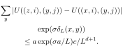
Searchable transcription

X
y
|U((z, i), (y, j)) −U((x, i), (y, j))|
exp(σδL(x, y))
≤a exp(σa/L)c/Ld+1.

Searchable transcription

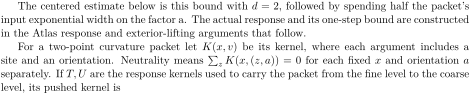
The centered estimate below is this bound with d = 2, followed by spending half the packet’s
input exponential width on the factor a. The actual response and its one-step bound are constructed
in the Atlas response and exterior-lifting arguments that follow.
For a two-point curvature packet let K(x, v) be its kernel, where each argument includes a
site and an orientation. Neutrality means P
z K(x, (z, a)) = 0 for each fixed x and orientation a
separately. If T, U are the response kernels used to carry the packet from the fine level to the coarse
level, its pushed kernel is

Searchable transcription

K′(y, z) =
X
x,v
T(x, y)K(x, v)U(v, z).

All rearrangements below use absolute convergence. It follows from the packet’s weighted row bound and the row and column bounds on T,U: first sum the nonnegative absolute majorant in the output variables, then in the input variables. The resulting finite product of bounds dominates the full multiple series. Thus both iterated sums and regrouping by the finite orientation sets are justified.

Neutrality removes the spatially constant part of the right response. For fixed, replace bysiteorientation)). The removed sum vanishes separately for each orientation. If = dist(sitesite), the spatial difference estimate gains relative to the ordinary row estimate. For positive input width and output width with 2

Searchable transcription

a exp(σa/L) ≤(2/τ) exp(τa).

Indeed2, and) exp(2), the latter following fromexp() for The centered right row therefore costs for a degree-two predictor of cost c. The held left column costs. Multiplication, followed by the input packet bound p, gives

Searchable transcription

foldedσ(K′) ≤[|α|q|β|(2/τ)c/L]p.

This is the precise neutralCoin factor used in the flat recursion. The gain comes from centering before taking absolute values. The secured pilot and wire bounds in this chapter provide the predictor spatial difference estimate.

Searchable transcription

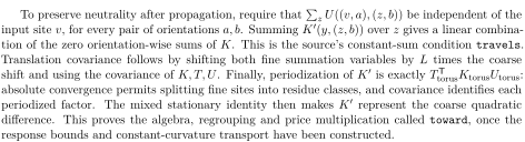
To preserve neutrality after propagation, require that P
z U((v, a), (z, b)) be independent of the
input site v, for every pair of orientations a, b. Summing K′(y, (z, b)) over z gives a linear combina-
tion of the zero orientation-wise sums of K. This is the source’s constant-sum condition travels.
Translation covariance follows by shifting both fine summation variables by L times the coarse
shift and using the covariance of K, T, U. Finally, periodization of K′ is exactly T T
torusKtorusUtorus:
absolute convergence permits splitting fine sites into residue classes, and covariance identifies each
periodized factor. The mixed stationary identity then makes K′ represent the coarse quadratic
difference. This proves the algebra, regrouping and price multiplication called toward, once the
response bounds and constant-curvature transport have been constructed.

Positive three-form correction

The linear flight construction uses a matrix symbol on the whole three-form coordinate space of the form

Searchable transcription

A = V + lI −mS∗S,

Here0 is the fine amendment parameter and the coarse parameter. On real momentum the symbols are Hermitian. The analytic estimates give and, where is a fixed orientation-count constant, 0 depend only on the smoothing pair and penalty, and is the block length. Choose + 2 and require. Then, for every vector

Searchable transcription

⟨x, Ax⟩≥[−a2C + l −ma2B/L2]∥x∥2 ≥∥x∥2.

This is positivity on the full three-form space. No restriction to the image of the exterior derivative is used to obtain it. For the corrected form, a uniform inverse bound yields. The source obtains W from a uniformly bounded right inverse of F, which in these square finite matrices is also a left inverse. An independent analytic row estimate supplies the upper bound. This explains why the coarse amendment threshold is chosen before the fine block length, while the subsequent length condition absorbs the already fixed fine amendment.

The rebased correction identity has the following exact content. Let X,Y be the fine and coarse amended inverse metrics, B the coarse amended metric, T the installed inverse response, and the coarse exterior derivatives. Then

Searchable transcription

B[Y −T TXT −b−1d1dT
1 ]B = dT
2 Rd2.

Searchable transcription

To derive this, write Y = B0 + lRT
0 R0 and X = b0 + mF T
0 F0. The unamended defect is RT
0 V R0
and the intertwining identity is SR0 = F0T. Substitution makes the bracket RT
0 (V +lI −mSTS)R0.
Since R0B = Fd2 and B is symmetric, the displayed formula follows with R = F TAF. The exterior
lifts, regular symbols and analytic inverse estimates construct B0, b0, S, F with the bounds used
here.

Roots for the bottom metric

Searchable transcription

Let the amended metric M have real-axis lower bound b0I, and choose the clip coefficient 0 < c ≤
b0/2. Then M −cI ≥(b0/2)I. Subtracting the constant row cI preserves the analytic strip bound.
The positive analytic-root construction gives a real Laurent row F with F TF = M −cI on every
finite torus. Adjoin the constant block √c I. Its Gram matrix is exactly