Quantum Source Completions and Memory–Environment Tradeoffs
Stationary quantum completions and the readout interface
Stationary quantum completions and the readout interface

Searchable transcription
A nonnegative stationary triple array p(i, y, j) has middle slices My(i, j) = p(i, y, j) and adjacent masses
w(i, y) = ∑︁
j p(i, y, j) = ∑︁
k p(k, i, y). The classical deterministic-readout minimum ∑︁
y rank+(My) is
an existing comparison theorem, not claimed as a new result here. The exact classical comparison is

Searchable transcription
Nmin(p) =
∑︂
y
rank+(My),
(1)
with its full stationary gluing proof established in Rodgers [12]. We give its quantum counterpart in a distinct orthogonal-current-symbol class, then distinguish that class from general emitted-symbol instruments.
The exact quantum completion theorem
Let ) be a normalized stationary triple array on a finite alphabet:

Searchable transcription
w(i, y) :=
∑︂
j
p(i, y, j) =
∑︂
k
p(k, i, y).
(2)

Searchable transcription
Omit symbols with zero stationary probability. Write rankC
psd(M) for the least d admitting d-dimensional
complex Hermitian PSD factors Mij = Tr(AiBj). Positive-semidefinite rank and its static correlation-
generation interpretation are established[4, 6]; the additional requirement below is one stationary
recurrent source, not a separate factorization for each observation.

Searchable transcription
The declared source class has a Hilbert space H = ⨁︁
y Hy, block-diagonal memory states, and
current readout y given by its orthogonal sector. A time-homogeneous Markov step is specified by CP
maps
Φj←y : B(Hy) −→B(Hj),
∑︂
j
Φ∗
j←y(I) = I.

Searchable transcription
Reading the sector projectively does not change a block-diagonal state. The source cost is the total
Hilbert dimension D = ∑︁
y dim Hy, including its visible current-symbol register. An open Markov
channel, with fresh environment degrees of freedom at each step, is allowed explicitly. This parallels the
fresh randomness allowed in a classical stochastic Markov source; it is not a count of all environmental
or archival degrees of freedom in a closed universe.
Theorem 2.1 (Exact quantum completion with orthogonal current readout). In the declared source class the exact minimum for the triple array is

Searchable transcription
y
rankC
psd(My).
(3)
Dmin(p) =
∑︂
An optimum can be chosen with measure-and-prepare block channels. It realizes the entire canonical stationary order-two completion of . Consequently, for a specified full stationary order-two law, the same expression is its exact minimum in this class. No full-law claim for higher-order input processes is made.

Searchable transcription
Proof. For the lower bound let τy be the stationary positive block of an arbitrary admissible source,
with ∑︁
y Tr τy = 1. Put
Ay
i = Φy←i(τi),
By
j = Φ∗
j←y(I).

Searchable transcription
Both are positive and p(i, y, j) = Tr(Ay
i By
j ). Hence each sector dimension is at least its slice’s complex
PSD rank; summation proves the bound.
For attainment choose minimum PSD factors separately in each sector. They may be normalized
without increasing their dimensions. Specifically, set Sy = ∑︁
j By
j , restrict to its support, and replace

Searchable transcription
Ay
i ↦−→S1/2
y
Ay
i S1/2
y
,
By
j ↦−→S−1/2
y
By
j S−1/2
y

Searchable transcription
on that support. Cyclicity of trace and support of every By
j preserve all pairings, while ∑︁
j By
j = I.
Thus Tr Ay
i = w(i, y). Define τy = ∑︁
i Ay
i and restrict further to its support, compressing all factors
there. Pairings and the effect sum are again preserved, and τy is now faithful. Since

Searchable transcription
Tr(By
j τy) =
∑︂
i
p(i, y, j) = w(y, j),

Searchable transcription
a zero w(y, j) implies By
j = 0 on this support. The destination matrix Aj
y also vanishes because its
trace is w(y, j).
For positive w(y, j) set

Searchable transcription
σj
y =
Aj
y
w(y, j),
Φj←y(X) = Tr(By
j X)σj
y;
(4)

Searchable transcription
set the map to zero otherwise. These are CP maps with effects By
j , so each input sector’s summed
map is trace preserving. The constructed state is stationary because
∑︂
y
Φj←y(τy) =
∑︂
y
Aj
y = τj.

Searchable transcription
It is normalized since ∑︁
y Tr τy = ∑︁
i,y w(i, y) = 1. After any positive-probability observed pair (i, y)
the normalized memory state is exactly σy
i . Its next-output law and next state are

Searchable transcription
Pr(j | i, y) = Tr(By
j σy
i ) = p(i, y, j)
w(i, y) ,
σj
y.
The channel therefore gives, for

Searchable transcription
n−1
∏︂
p(yt−1, yt, yt+1)
Pr(y1 · · · yn) = w(y1, y2)
w(yt−1, yt)
.
(5)
t=2
Forbidden transitions have probability zero; no division is used along them. This is the canonical order-two word law. Support reductions cannot strictly reduce the final dimension below a slice’s minimum PSD rank, by the already proved lower bound. Equality follows.
The arbitrary-past quantum conditional state in this theorem need not be perfectly distinguishable from the states induced by other pasts. That is the source of the compression. Neither exact recovery of the past symbol nor preservation of all inaccessible purifying records is asserted.
A full-support, strictly smaller quantum realization
For a finite circular phase representation, informed by the geometric phase and angular-register descriptions in [8, abstract and Sections 2–3] and [9, pp. 64–68], use the following quantum encoding and symbol maps. Let cos
 sin
 0), and let
 be the Pauli matrices. For a dimensionless noise parameter 0
 1, define

Searchable transcription
ρi = I + ni · σ
2
,
Eλ
j = I −(1 −λ)nj · σ
3
.
(6)
The states are pure; the effects are positive and sum to identity. The probability matrix is

Searchable transcription
{︄
λ/3
i = j,
1/2 −λ/6
i ̸= j.
(7)
T λ
ij = Tr(Eλ
j ρi) = 1 −(1 −λ) cos(θi −θj)
3
=
It is symmetric doubly stochastic with eigenvalues 1 2. Interleave two independent stationary
 -chains. Their full law is

Searchable transcription
n−2
∏︂
Pr(y1 · · · yn) = 1
t=1
T λ
yt,yt+2,
n ≥2.
(8)
9

Searchable transcription
Every finite word is positive when 0 < λ < 1; the noiseless model has forbidden events Yt+2 = Yt.
Adjacent pairs are uniform for all these models.
Each triple slice is My = T λ/9. It has ordinary rank three, so its nonnegative rank is exactly three.
The quantum factors Ay
i = ρi/9, By
j = Eλ
j have size two, and PSD rank one would force ordinary rank
one. Hence Theorem 2.1 and the classical baseline give the exact comparison

Searchable transcription
Dsector = 6,
Nclassical,det = 9.
(9)

Searchable transcription
The explicit channel is Φj←y(X) = Tr(Eλ
j X)ρy with stationary blocks τy = I/6. Thus the reduced
memory is the physical state of one qubit inside each of three orthogonal current-output sectors; no
hidden classical controller remembering the preceding label is permitted in the resource count.
For the full law, nine is also the exact minimum among all finite classical HMMs with memoryless stochastic emissions: their past-two/future-two joint matrix factors through the hidden state, whereas here

Searchable transcription
H(a,b),(c,d) = T λ
acT λ
bd
9
= (T λ ⊗T λ)(a,b),(c,d)
9
(10)
has rank nine. A nine-state causal-pair source attains the law. This is a use of Rodgers’s existing Hankel-rank method, not a newly invented lower-bound method. There is a finite-data margin. The smallest singular value of each 18. If a normalized triple distribution
 satisfies TV
 36, then each slice perturbation has operator norm at most its entrywise
 norm, at most 2 TV
 ), and every perturbed slice retains rank three. Consequently every deterministic-instantaneous classical source reproducing
 still needs at least nine states. For arbitrary stochastic emissions, the four-time version follows from
 four-time TV error less than (1
 72 retains the rank-nine lower bound. These are dimension certificates under their respective source interfaces, not device-independent claims that an unknown apparatus has quantum memory.
Circular grids of arbitrary resolution
For any 3 use equally spaced phases
 and the same pure states
 . Define

Searchable transcription
Ej = I −nj · σ
m
,
Tij = 1 −cos(θi −θj)
m
.
(11)

Searchable transcription
The POVM is normalized because ∑︁
j nj = 0. The transition is symmetric doubly stochastic, has zero
diagonal and strictly positive off-diagonal entries, and has rank three. To check its rank explicitly,
write ci = cos θi, si = sin θi. Then

Searchable transcription
T = J −ccT −ssT
m
,

Searchable transcription
and the mutually orthogonal vectors 1, c, s have squared norms m, m/2, m/2. The three nonzero
eigenvalues are 1, −1/2, −1/2. The order-two law is m−2 ∏︁
t Tyt,yt+2. Every triple slice has PSD rank
exactly two; its exact quantum sector cost is 2m.

Searchable transcription
Proposition 2.2 (Classical sector cost grows with angular resolution). Let rm be the smallest integer
r with m ≤
(︁
r
⌊r/2⌋
)︁. Every classical deterministic-instantaneous source for the phase-circle triple law
has at least mrm states.

Searchable transcription
Proof. In any nonnegative factorization T = AB with r factors let Si = {l: Ail> 0}. If Si ⊆Sj, the
zero Tjj implies Blj = 0 for every l∈Sj, hence Tij = 0. This contradicts Tij > 0 for i ̸= j. Thus the
m supports are an antichain. To recall the counting bound without relying on a citation, a uniformly
random permutation of r elements has at most one initial segment belonging to an antichain. A set S
is such an initial segment with probability
(︁r
|S|
)︁−1. Taking expectations yields ∑︁
i
(︁r
|Si|
)︁−1 ≤1, hence
m ≤
(︁
r
⌊r/2⌋
)︁, the classical Sperner bound[14]. Apply this to every slice of (1).
Phase count
 Quantum sector minimum Classical sector lower bound

Searchable transcription
180
10
360
1800
360
11
720
3960
720
12
1440
8640
The grid sizes follow the finite angular registers in [9, pp. 64–68]; the probabilities are those of the instrument defined here, not inferred from geometric line density. The classical values are lower bounds,
not asserted exact nonnegative ranks. Known low-PSD-rank/high-nonnegative-rank distance geometry already supplies the static phenomenon; the added stationary channel realizes it at every time and proves the full observed law.
Removing the stored classical output: exactly two qubits
The sector restriction matters. A general iterated quantum instrument may emit the current output into an external archive without preserving it in an orthogonal sector of the internal memory. In this broader class a quantum source consists of a density matrix on , CP maps Ψ
 whose sum is trace preserving, and a stationary density matrix. Word probabilities are traces of successive maps. All outputs are retained; no null, failure or loss outcome is postselected away.
Theorem 2.3 (Exact emitted-symbol instrument dimension). For every noiseless phase-circle law (11) , the minimum internal Hilbert dimension among stationary iterated quantum instruments is exactly four.
Proof. For attainment use two qubits and define

Searchable transcription
Ψj(X) = Tr1[(Ej ⊗I)X] ⊗ρj.
(12)

Searchable transcription
The partial trace equals the result of sandwiching X by
√︁Ej ⊗I before tracing the first qubit, so this
is CP. Its effect is Ej ⊗I; summing the effects gives identity. On product inputs,

Searchable transcription
Ψj(ρa ⊗ρb) = Tajρb ⊗ρj.
Starting from 4, the first two outputs are independent uniform symbols; the conditional memory then equals
 . Every later step emits
 with probability
 and shifts the two states. This proves every finite word of the target law, with no accumulated approximation. Also

Searchable transcription
I2
2m ⊗ρj = I4/4,
∑︂
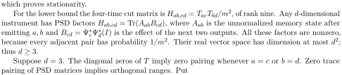
j
Ψj(I4/4) =
∑︂
j
Searchable transcription
which proves stationarity.
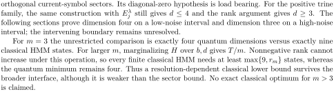
For the lower bound the four-time cut matrix is Hab,cd = TacTbd/m2, of rank nine. Any d-dimensional
instrument has PSD factors Hab,cd = Tr(AabBcd), where Aab is the unnormalized memory state after
emitting a, b and Bcd = Ψ∗
cΨ∗
d(I) is the effect of the next two outputs. All these factors are nonzero,
because every adjacent pair has probability 1/m2. Their real vector space has dimension at most d2;
thus d ≥3.
Suppose d = 3. The diagonal zeros of T imply zero pairing whenever a = c or b = d. Zero trace
pairing of PSD matrices implies orthogonal ranges. Put
 = span
 ran

 = span
 ran

The nonzero range of is orthogonal to
 dim
 2 for every
 . If some
 has dimension two, every
 , and all effects
 are supported on that same two-dimensional subspace. Compressing all factors to it gives rank
 4, contradicting nine. The same reasoning excludes a two-dimensional
 . Otherwise all these nonzero spaces are lines. Since every
 = 0 has range contained in both
 and
 , all lines are equal; this would give rank at most one, another contradiction. Therefore
 = 3 is impossible, and the four-dimensional construction is optimal.

Searchable transcription
The theorem gives a completed dimension lower bound beyond the generic
√
rank estimate. It holds for arbitrary complex quantum instruments, not only for the particular shift update or for
Searchable transcription
orthogonal current-symbol sectors. Its diagonal-zero hypothesis is load bearing. For the positive trine
family, the same construction with Eλ
j still gives d ≤4 and the rank argument gives d ≥3. The
following sections prove dimension four on a low-noise interval and dimension three on a high-noise
interval; the intervening boundary remains unresolved.
For m = 3 the unrestricted comparison is exactly four quantum dimensions versus exactly nine
classical HMM states. For larger m, marginalizing H over b, d gives T/m. Nonnegative rank cannot
increase under this operation, so every finite classical HMM needs at least max{9, rm} states, whereas
the quantum minimum remains four. Thus a resolution-dependent classical lower bound survives the
broader interface, although it is weaker than the sector bound. No exact classical optimum for m > 3
is claimed.