Preparation uncertainty and a sharp conditional-error frontier

Preparation uncertainty and a sharp conditional-error frontier

Uncertainty and the unchanged access contract

Use two degenerate one-excitation source modes. The unknown label is. Its source marginal belongs to

Searchable transcription

(︄
p
hv
√︁
)︄
p(1 −p)e−iδ
ρh(p, δ, v) =
,
p ∈[p−, p+],
|δ| ≤∆,
v ∈[v−, 1],
(17)
hv
√︁
p(1 −p)eiδ
1 −p

where 01 and 0∆2. Both labels have the same mode intensities. The width in is source-amplitude uncertainty; is source visibility, which may arise from correlations with a retained inaccessible environment. An unknown reader phase offset can be included in ∆by adding its bounded offset to the source phase interval, provided the resulting halfwidth is at most

2. Separate finite calibration procedures can supply these bounds, but they are assumptions of this theorem. No future sample or statistical independence is inferred from a calibration trace. The physical apparatus is exactly the coherent conversion model’s ready subspace plus two stable flags. Its Hamiltonian is

Searchable transcription

(︄
A(t)
C(t)∗
)︄
H(t) = ħ
,
∥C(t)∥≤G,
C(t)
D(t)

with Hermitian block controls. Uniform ready-subspace loss at ratetransfers the source state isometrically into orthogonal retained output modes. The bath starts in its vacuum, all preparations are independent of the unknown input, and there is no re-excitation or additional protected storage. andhave units s; the deadline is in seconds. Source plus arbitrary inert reference may be in any joint state with marginal (17). The reference is retained and unread. The lost bath, surviving source and null flag are also retained but are inconclusive to this fixed stable-flag readout catalogue. A new coherent bath reader or a procedure reporting guesses on a null outcome changes the allowed decision problem. The two physical stable flags, observed only after the active coupling is off, are the only conclusive outcomes here. Let 1] be the coherent conversion model’s optimal transfer ceiling:

Searchable transcription

η = fG(τ)2,
τ = min(T, t∗).
(18)

Searchable transcription

For l< 4G,
fG(t) = G
G2 −l2/16,
t∗= arctan(4Ω/l)
Ωe−lt/4 sin(Ωt),
Ω=
√︂
Ω
.

Searchable transcription

At l= 0 take t∗= π/(2G). At l= 4G, use fG(t) = Gte−Gt, t∗= 1/G. For l> 4G, replace sine
by hyperbolic sine and Ωby χ =
√︁

, with artanh. The previously proved amplitude barrier implies, for every allowed control,

Searchable transcription

E+ + E−≤ηI,
(19)

because each input’s flag probability is at most. For completeness, its proof can be stated briefly. Split any no-loss vector into ready/flag norms cos sin Then ̇cos2 and ̇ 2) sin cos with. For

Searchable transcription

0
lcos2 u
G + (l/2) sin u cos udu,
F(θ) =
∫︂θ

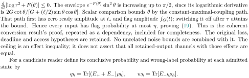
Searchable transcription

d
dt[log r2 + F(θ)] ≤0. The envelope e−F(θ) sin2 θ is increasing up to π/2, since its logarithmic derivative
is 2G cot θ/[G + (l/2) sin θ cos θ]. Scalar comparison bounds θ by the constant-maximal-coupling path.
That path first has zero ready amplitude at t∗and flag amplitude fG(t); switching it off after τ attains
the bound. Hence every input has flag probability at most η, proving (19). This is the coherent
conversion result’s proof, repeated as a dependency, included for completeness. The original loss,
deadline and access hypotheses are retained. No unrelated noise bounds are combined with it. The
ceiling is an effect inequality; it does not assert that all retained-output channels with those effects are
equal.
For a candidate reader define its conclusive probability and wrong-label probability at each admitted
state by
qh = Tr[(E+ + E−)ρh],
wh = Tr[E−hρh].

The objective is to maximize a guaranteed such that, for every

Searchable transcription

qh ≥Q,
wh ≤εqh.
(20)

Thus bounds the error conditioned on a conclusive record explicitly pays for that selection. No label prior is needed. The error condition is linear in the effects even on a zero-probability branch, where it is simply 0

Exact minimax solution

Searchable transcription

Put

Searchable transcription

2 log(ξ+/ξ−),
εmin = 1 −m sech w
m = v−cos ∆,
ξ± =
√︂
p±/(1 −p±),
w = 1
2
.
(21)

All these quantities are dimensionless. The logarithm is a log-amplitude-odds coordinate, not a new physical geometry.

Proposition 3.1 (Sharp robust conditional-error/conclusive frontier). If, no positive guaran- teed conclusive probability satisfies (20). The zero-conclusive reader is still allowed. For and , define

Searchable transcription

hε = arcosh
m
1 −2ε,
L = −hε −log ξ−,
U = hε −log ξ+.
(22)

The interval is nonempty. Letbe its point nearest zero and put. Then the exact maximum is

Searchable transcription

Qmax = η minp∈{p−,p+}[pr2 + 1 −p]
max(1, r2)
.
(23)

Searchable transcription

It is attained by the effects

Searchable transcription

(︄
x
±√xy
±√xy
y
x =
ηr2
)︄
max(1, r2),
y =
η
max(1, r2),
E± = 1
.
(24)
2

For attains, positive conclusive probability requires These are optima within the declared stable-flag catalogue, not over readings of every retained output.

Proof. First enlarge the physical set to all positive effects satisfying (19). This can only raise the optimum. The source set is invariant under diag1) with label exchange and under complex conjugation with. Averaging the candidate effects with these two transformations preserves all linear constraints (20). Thus an optimum in this enlarged set may be taken as

Searchable transcription

(︄
x
±z
±z
y
)︄
,
0 ≤x, y ≤η,
z2 ≤xy,
z real.
E± = 1
2

Searchable transcription

This averaging is an upper-bound argument about effects; it introduces no unaccounted physical coin
or protected register. Because cos δ ≥0 and v ≥0, replacing z by √xy reduces every wrong probability
without changing any conclusive probability. Therefore the rank-one form (24) suffices in the relaxation.
For positive x, y set r =
√︁

. The worst phase and visibility are. At a specified

Searchable transcription

q(p) = px + (1 −p)y,
[︄
]︄
w(p)
1 −2m
√︁
p(1 −p)xy
px + (1 −p)y
q(p) = 1
= 1
2[1 −m sech(log r + log ξ(p))].
(25)
2

Searchable transcription

A reader with x = 0 or y = 0 has conditional error 1/2 whenever it clicks; it cannot improve the case
ε < 1/2. The least contrast in (25) occurs at an endpoint of the log-odds interval. Balancing its two
endpoint distances gives the unique minimum possible worst distance w, proving (21). At the floor the
optimal ratio obeys log r = −1
2 log(ξ−ξ+).

For an error tolerance at or above the floor, the requirement is precisely

Searchable transcription

| log r + log ξ(p)| ≤hε
for all p,

which is (22). At fixed, error is independent of the common scale. Maximal conclusive probability therefore uses the largest scale allowed by. For1 its guaranteed probability is ], strictly increasing with. For], strictly decreasing with . The point of the admissible log interval nearest zero is thus optimal, proving (23) in the relaxation. The following construction attains those effects in the actual apparatus, so the upper bound is sharp for the physical model as well. The = 0 and2 boundary cases follow directly from (25) and (19).

This yields a precise obstruction and its useful repair. Robust zero error with positive success is possible only when = 1 and the amplitude interval is a single point. With any genuine amplitude width, visibility loss or phase width, one must either abstain always or allow a positive error. For the point case

Searchable transcription

r2 = (1 −p)/p,
Qmax = 2η min(p, 1 −p),

recovering the coherent conversion model’s exact unambiguous reader. With2, the error floor is (12 and no amplitude filter improves it.

Attaining interaction, complete outputs and the loss frontier

Searchable transcription

Let H = 2−1/2(︁1 1
1 −1
)︁and use, during τ,
A = D = 0,
C = H diag(gx, gy),
fgx(τ) = √x,
fgy(τ) = √y.
(26)

Searchable transcription

The coherent conversion model’s damped transfer amplitude at coupling g is continuous on [0, G],
equals zero at g = 0 and equals √η at g = G. Since x, y ≤η, both required couplings exist by the
intermediate-value theorem. The coupling is fixed before the unknown input, uses no actual-sign
feedback, has ∥C∥≤G, and hence has cross-subspace Hamiltonian norm at most ħG. Switch it off
after τ; the flags then remain untouched until the deadline T. The terminal conclusive maps are exactly

Searchable transcription

K+ = −i
√
2|+⟩(√x⟨0| + √y⟨1|),
K−= −i
√
2|−⟩(√x⟨0| −√y⟨1|).
(27)

Searchable transcription

They reproduce (24) for every source-reference input, not only for the designated family.
For full bookkeeping let V (t) = exp[(−iH/ħ−lPR/2)t]IR on the active interval. The surviving-
source map is K0 = e−l(T−τ)/2PRV (τ). Lost quantum outputs have maps Kloss(t) =
√

) for , and the freely decaying ready remainder gives the corresponding maps for. They obey

Searchable transcription

K∗
0K0 + K∗
+K+ + K∗
−K−+
∫︂T
0
Kloss(t)∗Kloss(t)dt = I.

The isometries transport the instantaneous lost two-mode component, including its conditional correlations with. Earlier filtering and conditioning need not preserve the original input correlations. No failure is removed or redrawn. Tensoring each map with defines the complete retained instrument. Coherent bath output and a measured time archive are alternative output choices; extra physical classicalization environments are not included in a four-mode count for the active Hamiltonian. The attained reader has phase-independent conclusive, null and loss probabilities at specified

Searchable transcription

q(p) = px + (1 −p)y,
n(p) = pnx + (1 −p)ny,
l(p) = 1 −q(p) −n(p),

where and is the ready amplitude of the damped tap. Thus loss and null remain separately predictable and retained. The theorem optimizes conclusive probability under an error constraint; it does not additionally minimize lost mass among every possible realization of the same effects. Write, with determined entirely by the source uncertainty and chosen error budget. A required guaranteed rateis feasible exactly when

Searchable transcription

ε ≥εmin,
η(G, l, T)B ≥Q∗.
(28)

This is a sharp physical loss/control requirement within the same model. It keeps the preparation penalty separate from the independently specified loss/control factor. It does not join a visibility parameter from one noise model to an incompatible apparatus bound. For a deadline at least the first transfer peak, gives an explicit one-variable loss threshold.

An exact extension for uncertain mode efficiencies

A calibrated efficiency interval can be treated without pretending that it is uncertainty in the entire Hamiltonian. Put an unknown but fixed two-mode attenuator before every reader control, with

Searchable transcription

β),
Bαβ = W diag(
√
Aαβ = diag(√α,
√︁
1 −α,
√︁
1 −β),

Searchable transcription

where W maps into two retained upstream-loss modes and A∗
αβAαβ + B∗
αβBαβ = I. Assume Cartesian
bounds 0 < α−≤α ≤α+ ≤1 and 0 < β−≤β ≤β+ ≤1. There is no statistical independence
assumption on these device parameters.
They are not refreshed following loss, and there is no
compensating input-dependent control before the attenuator or conclusive reader of its lost modes.

Proposition 3.2 (Sharp uncertainty in upstream path transmission). The preceding solution remains exact after replacing the log-odds interval [log log by

Searchable transcription

t−= log ξ−+ 1
2 log(α−/β+),
t+ = log ξ+ + 1
2 log(α+/β−).

Its conditional-error floor is sech. For a feasible, choose log nearest zero in. The exact guaranteed probability on the original trial population is

Searchable transcription

Qeff
max =
η
max(1, r2)
min
p∈{p−,p+}[pα−r2 + (1 −p)β−].
(29)

Proof. The actual conclusive probability is. Its conditional contrast is sech(log log

log)). The possible argument is exactly the interval just stated, so the same endpoint minimax calculation gives the conditional-error constraint. Conclusive probability is smallest at and an endpoint of. At maximum allowed scale its value is increasing in for1 and decreasing for 1, for each separately and hence also for their minimum. This proves (29). The relaxed-POVM upper-bound proof and the actual attaining post-attenuation pulse are unchanged. Every downstream Kraus map is now multiplied on the right by, and is a further retained quantum branch. Completeness therefore remains exact on arbitrary references. No normalization by the probability of upstream survival has been silently performed.

For the example below, adding 1] raises the conditional-error floor from 0 08, it reduces guaranteed conclusive probability from 0 1656759538, attained by gains5062765525. This is a sharp reader with uncertain path transmission, not an approximate bound on arbitrary gain miscalibration. Uncertain scalar lifetime or coherent coupling is a different interface and is held open here. The physical-threshold curve (28) permits redesign at each known; it is not one pulse certified for an

unknown range of. Indeed the fixed eight-percent pulse designed at= 1 below has worst conditional error 008016304046 if the actual rate is 08. Less loss changes the relative transfer amplitudes and can increase the conditional error. Substituting a worst-case while keeping its nominal optimal ratio would therefore be invalid. A joint calibrated effect region or an additional robust-control optimization is needed for that task.