Bounded coherent conversion and complete detector records

Bounded coherent conversion and complete detector records

Source and declared apparatus

Use two degenerate source modes, with a single excitation spanning span. The two possible source states are

Searchable transcription

|ψ±⟩= a|0⟩± b|1⟩,
a =
√︂
(1 + s)/2,
b =
√︂
(1 −s)/2,
0 < s < 1.
(1)

They have the same separate mode intensities and overlap. Their relative phase differs by. Using normalized phase-sensitive templates, informed by [7, pp. 18–21, Eqs. (58)–(70)] and [8, Section 32, pp. 42–43], define the reciprocal reader states

Searchable transcription

|φ±⟩= b|0⟩± a|1⟩,
⟨φ±|ψ∓⟩= 0,
|⟨φ±|ψ±⟩|2 = 1 −s2.

The readout has two orthogonal, stable flag modes labelled + and. There are also orthogonal lost-output modes, initially vacant. Every mode is included in the one-excitation description; no new actual sample is loaded after a null result. Source/reference inputs can be any with arbitrary finite inert reference. The reader and vacant output modes have one common input-independent preparation. The loss bath starts in its vacuum, independently of that original preparation; the scalar Markov loss law and absence of re-excitation are physical model assumptions of the declared apparatus. The claim of unambiguity is for the designated pair (1); the instrument itself is defined for every reference-extended input. The apparatus Hamiltonian on the ready-plus-flag subspace is

Searchable transcription

(︄
A(t)
C(t)∗
)︄
H(t) = ħ
,
A = A∗,
D = D∗,
∥C(t)∥≤G.
(2)
C(t)
D(t)

Searchable transcription

A, C, D are piecewise continuous on the finite control interval; the stated bound holds almost everywhere.
This regularity ensures that the propagator below exists. G > 0, A, C, D have units s−1 and H has
units joules. Uniform irreversible loss acts only on the ready subspace at rate l≥0 in s−1. Its complete
amplitude map is Lloss =
√

, where is an isometry to the lost-output space. It isometrically transports the instantaneous ready component, including its conditional reference assemblage. Earlier filtering and conditioning may have changed the original source/reference correlations; no preservation of those original correlations is asserted. The outgoing state is not replaced by a vacuum or a classical label. Once lost, the excitation never returns. There are no other protected storage subspaces, fresh inputs, gain channels or readers of the lost field in the allowed conclusive-record catalogue. Block Hamiltonians are allowed in the upper bound; they cannot be used to add an uncounted protected

ancilla. The optical/cavity coupling and its timing are prescribed controls; this is not an autonomous clock construction. The no-loss propagator on the four-dimensional ready-plus-flag space is

Searchable transcription

 ̇Ueff(t) = [−iH(t)/ħ−lPR/2] Ueff(t).

Let embed the two-dimensional source. A complete terminal instrument consists of

Searchable transcription

K± = P±Ueff(T)IR,
K0 = PRUeff(T)IR,
Kloss(t) =
√
lWtPRUeff(t)IR.
(3)

Here retains the outgoing quantum mode. The coherent temporal output is an amplitude sector; a registered loss time is instead a classical record, with the output-space convention specified below. The identity

Searchable transcription

K∗
0K0 + K∗
+K+ + K∗
−K−+
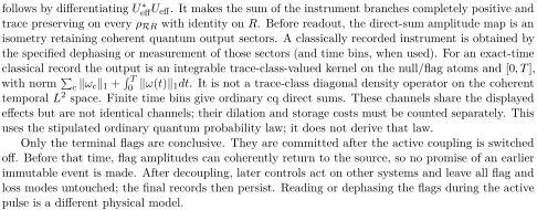
∫︂T
0
Kloss(t)∗Kloss(t)dt = I
(4)

Searchable transcription

follows by differentiating U∗
effUeff. It makes the sum of the instrument branches completely positive and
trace preserving on every ρRR with identity on R. Before readout, the direct-sum amplitude map is an
isometry retaining coherent quantum output sectors. A classically recorded instrument is obtained by
the specified dephasing or measurement of those sectors (and time bins, when used). For an exact-time
classical record the output is an integrable trace-class-valued kernel on the null/flag atoms and [0, T],
with norm ∑︁
c ∥ωc∥1 +
∫︁T
0 ∥ω(t)∥1dt. It is not a trace-class diagonal density operator on the coherent
temporal L2 space. Finite time bins give ordinary cq direct sums. These channels share the displayed
effects but are not identical channels; their dilation and storage costs must be counted separately. This
uses the stipulated ordinary quantum probability law; it does not derive that law.
Only the terminal flags are conclusive. They are committed after the active coupling is switched
off. Before that time, flag amplitudes can coherently return to the source, so no promise of an earlier
immutable event is made. After decoupling, later controls act on other systems and leave all flag and
loss modes untouched; the final records then persist. Reading or dephasing the flags during the active
pulse is a different physical model.

Sharp finite-lifetime success frontier

For a two-dimensional input, error-free conclusive effects necessarily have

Searchable transcription

E± = K∗
±K± =
q±
1 −s2 |φ±⟩⟨φ±|,
 ̄q = (q+ + q−)/2.
(5)

This follows because a positive effect with zero expectation inannihilates that vector. In particular,

Searchable transcription

⟨1|(E+ + E−)|1⟩=
 ̄q
1 −s.
(6)

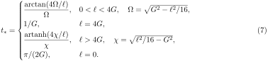
A bound on coherent transfer of the inputtherefore bounds the average success of every allowed unambiguous reader, including asymmetric ones. Defineby

Searchable transcription

⎧
⎪
⎪
⎪
⎪
⎪
⎪
⎪
⎪
⎨
arctan(4Ω/l)
G2 −l2/16,
Ω
,
0 < l< 4G,
Ω=
√︁
1/G,
l= 4G,
artanh(4χ/l)
t∗=
(7)
⎪
⎪
⎪
⎪
⎪
⎪
⎪
⎪
⎩
χ
,
l> 4G,
χ =
√︁
l2/16 −G2,
π/(2G),
l= 0.

Searchable transcription

Let τ = min(T, t∗) and
(G/Ω)e−lt/4 sin(Ωt),
l< 4G,
Gte−Gt,
l= 4G,
(G/χ)e−lt/4 sinh(χt),
l> 4G.
⎧
⎪
⎪
⎨
fG(t) =
(8)
⎪
⎪
⎩
The l= 0 first case has Ω= G.

Proposition 2.1 (Optimal phase-to-flag conversion with an independent loss sink). Under the declared apparatus and stable-flag readout catalogue,

Searchable transcription

 ̄q ≤(1 −s)fG(τ)2.
(9)

The bound is attained with. For a deadline at leastit is

Searchable transcription

qmax = (1 −s)e−lt∗/2.
(10)

It remains valid when arbitrary inert references and all original loss/null outputs are retained. It is not an optimum over new measurements of those retained outputs or of the reference.

Proof. First consider any normalized source input and its no-loss vector, split into ready and flag components with norms and. Write cos sin2. Loss gives ̇ cos2. Cauchy–Schwarz applied to the cross Hamiltonian gives an effective real transfer control with and ̇2) sin cos

Block Hamiltonians cancel from these norm equations. At zero components the same conclusions follow by continuous limits. Define

Searchable transcription

0
lcos2 u
G + (l/2) sin u cos u du.
F(θ) =
∫︂θ

For every trajectory, including controls that reverse direction,

Searchable transcription

d
dt[log r2 + F(θ)] = lcos2 θ
[︃geff + (l/2) sin θ cos θ
G + (l/2) sin θ cos θ −1
]︃
≤0.

Thus sin. This upper envelope increases on 02, since its logarithmic derivative is

Searchable transcription

2 cot θ −
lcos2 θ
G + (l/2) sin θ cos θ =
2G cot θ
G + (l/2) sin θ cos θ > 0.

Scalar comparison also bounds) by the trajectory with until that trajectory first reaches 2. Hence constant maximal coupling, stopped at that first time, maximizes flag transfer at every deadline. Its two scalar amplitudes are

Searchable transcription

uG(t) = e−lt/4[cos(Ωt) −lsin(Ωt)/(4Ω)],
vG(t) = −ifG(t),

Searchable transcription

with their continuous critical and hyperbolic forms. Its first ready zero is (7); at that time fG(t∗)2 =
e−lt∗/2. This proves the transfer bound y(T)2 ≤fG(τ)2. Apply it to |1⟩in (6) to obtain (9).
For attainability let H be the real balanced two-mode matrix 2−1/2(︁1 1
1 −1
)︁. Set A = D = 0 and,
during the active time τ,

Searchable transcription

√︄
1 −s
1 + s fG(τ).
(11)
C = H diag(g0, G),
fg0(τ) =

For = 0 the transfer amplitude is zero and for it is). Continuity in therefore guarantees a solution 0 to this intermediate target. No monotonicity assumption is needed. These are two independent damped taps in the balanced flag basis. Their terminal flag map is

Searchable transcription

−iH diag(fg0(τ), fG(τ)).

Equation (11) makes each wrong flag amplitude exactly zero for its excluded source state, and each correct probability equals (1. Switch off the coupling after; the stable flags then remain unchanged until. Residual ready amplitudes may subsequently be lost, and are included in (3). That proves attainability and preserves (4) on all inputs and their references.

Forand, one has, and 2025106210. The loss-limited transfer factor is 05062765525. Requiring success at least 2 with that overlap and a sufficiently long deadline gives the sharp threshold this apparatus class. Above it no permitted pulse sequence achieves the target. At the critical damping point, the transfer factor is; for large it is asymptotic to 4. For= 0 the frontier reduces to ideal unambiguous discrimination after a finite coherent pulse. These results are parameter requirements for a possible experiment, not measured biological lifetimes or coupling strengths.

Bounded coherent action and minimum output ranks

Searchable transcription

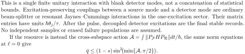
The loss-free implementation can be specified without a continuum bath. For any desired 0 ≤q ≤1 −s,
set
n0 =
√︂
1 −q/(1 + s),
n1 =
√︂
1 −q/(1 −s),
θj = arccos nj.

A constant four-mode Hamiltonian (2) with H diag( gives exactly

Searchable transcription

K0 = diag(n0, n1),
K± = −i
√︃
q
1 −s2 |±⟩⟨φ±|.
(12)

Searchable transcription

This is a single finite unitary interaction with blank detector modes, not a concatenation of statistical
bounds. Excitation-preserving couplings between a source mode and a detector mode are ordinary
beam-splitter or resonant Jaynes–Cummings interactions in the one-excitation sector. Their matrix
entries have units ħθj/τ. After the pulse, decoupled detector excitations are the final stable records.
No independent samples or erased failure populations are assumed.
If the resource is instead the cross-subspace action A =
∫︁∥PFHPR∥dt/ħ, the same norm equations
at l= 0 give
 ̄q ≤(1 −s) sin2(︁min{A, π/2}
)︁.

Searchable transcription

The construction saturates it, with A = arcsin
√︁

. This is a specialization of known unitary measurement resource bounds, included to make the physical resource contract explicit. Bounded Hamiltonian coupling is not the same constraint as a bounded Markov jump hazard; neither bound may be substituted into the other. For 0 the three terminal POVM effects have ranks 1 2 for + 0. Any orthogonal-record amplitude dilation of these exact effects requires at least 1 + 1 + 2 = 4 output dimensions: the amplitude map in each orthogonal record sector has rank equal to its effect. Equation (12) attains this count. At the null effect has rank one and the abstract minimum is three. The four-mode Hamiltonian is still a sufficient implementation; we do not claim it is a minimum-level Hamiltonian at that endpoint. Original input references tensor onto this count; they are not newly consumed reader ancillas. These are reachable orthogonal amplitude-sector dimensions. They do not include an extra pure environment needed to realize a fully dephased classical record channel; classicalizing a coherent flag requires its own retained-output accounting.

Why a static dark matched reader fails, and a continuous repair

Searchable transcription

Consider a static absorbing implementation of the matched-template prescription [7, pp. 18–21], with
fixed jump readers dark to the other source: L± = √γ |±⟩⟨φ±|. Initially the excluded click amplitude
is zero. However the full hazard is Q = γ diag(1 −s, 1 + s), so its null evolution changes the source.
For |ψ−⟩, the wrong + density at time t is

Searchable transcription

p+|−(t) = γa2b2[e−γ(1−s)t/2 −e−γ(1+s)t/2]2.
(13)

It is positive for 0. Its integrated infinite-time value is This is a tested obstruction to calling a fixed dark instantaneous kernel an error-free continuous instrument. A faithful repair keeps the reciprocal geometry and changes the reader to account for its own null back-action. Write

Searchable transcription

q(t) = (1 −s)(1 −e−κt),
N(t) = diag
(︃√︂
1 −q(t)/(1 −s)
)︃
,
1 −q(t)/(1 + s),
√︂

where 0 is a declared maximum signal hazard. Use

Searchable transcription

√︄
q′(t)
1 −s2 |±⟩⟨φ±|N(t)−1.
(14)
L±(t) =

At finite times these coefficients are bounded and known in advance. The Hamiltonian is zero; the reader does not acquire an actual sign to decide its next setting. Direct calculation gives

Searchable transcription

√︄
±
L∗
±L± = diag
(︃
q′
1 + s −q,
q′
q′(t)
1 −s2 |±⟩⟨φ±|.
)︃
≤κI,
L±(t)N(t) =
∑︂
1 −s −q

Searchable transcription

Thus every conclusive time is unambiguous. A null result filters the surviving quantum source, and the
predetermined reader compensates exactly for that filter. No fresh independence is inferred.
This bounded-hazard construction is also optimal in its own model class. For any absorbing two-port
unambiguous instrument with Q(t) ≤κI, the no-transition matrix satisfies N(t)∗N(t) ≥e−κtI, since
d
dt(N∗N) = −N∗QN ≥−κN∗N. With average cumulative success  ̄q(t), (6) gives

Searchable transcription

1 − ̄q(t)/(1 −s) = ⟨1|N(t)∗N(t)|1⟩≥e−κt.

Searchable transcription

Therefore  ̄q(t) ≤q(t), attained above, including when the two successes are allowed to be asymmetric.
Add independent uniform ready loss at rate l. The no-event matrix becomes e−lt/2N(t), the signal
Kraus density is e−lt/2L±(t)N(t) and the loss density is
√

). The three full effects plus the null effect sum to identity, as in (4). The optimal conclusive probability is

Searchable transcription

qhazard,loss(T) = (1 −s)
κ
κ + l[1 −e−(κ+l)T ].
(15)

Searchable transcription

To see optimality rather than only attainability, consider any competing schedule without loss and its
cumulative success qc(t) ≤q(t). Uniform loss multiplies its conclusive time density by e−lt. Integration
by parts gives
∫︂T
0
e−ltdqc(t) = e−lT qc(T) + l
∫︂T
0
e−ltqc(t)dt ≤
∫︂T
0
e−ltdq(t),

which is (15). This argument requires the same independent scalar loss law and the same stable conclusive-output catalogue; it does not combine unrelated noise models. At and = 2, the conclusive, null and loss probabilities are respectively 03967523953 and

A finite collision implementation and retained retry records

Searchable transcription

The continuous model has infinitely many temporal modes. A finite version need not pretend to
store such a continuum in a finite register. Choose M stages, tk = k∆, ∆= T/M, qk = q(tk) and
Nk = diag
√︁

Searchable transcription

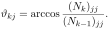
1 −qk/(1 ± s). At stage k, first attenuate both ready modes by e−l∆/2 into two fresh,
retained loss modes. Then use a two-mode tap with local null matrix NkN−1
k−1 and two fresh conclusive
modes. Its tap angles are

Searchable transcription

θkj = arccos (Nk)jj
(Nk−1)jj
.

The same finite Hamiltonian construction as (12) implements these taps and their balanced output mixing. Excitations already in old output modes never interact again. Consequently the cumulative null map is exactly, not a redraw. The conclusive Kraus maps in bin are

Searchable transcription

K±,k = e−ltk/2
√︄
qk −qk−1
1 −s2
|±, k⟩⟨φ±|,

Searchable transcription

and the loss map is
Kloss,k =
√︁
1 −e−l∆e−ltk−1/2WkNk−1.

Every original mode, source remainder and detector register is retained. These finite Kraus maps satisfy completeness exactly, for arbitrary inputs and inert references. They have success

Searchable transcription

M
∑︂
k=1
e−ltk(qk −qk−1),
e−l∆qhazard,loss ≤qM ≤qhazard,loss.
(16)
qM =

The bounds follow by bounding on each interval in the exact integral. This is a probability convergence guarantee; no equality of the unmeasured continuum bath and the finite bath is asserted. For the numerical example above = 8 gives2842794177, and = 128 gives 0 For positive loss and finite nonzero stages, each of the 2 conclusive effects has rank one, each of the loss effects rank two, and the null effect rank two. An orthogonal time-bin record dilation thus needs at least 4 + 2 reachable output dimensions; the one-excitation mode construction has exactly that count. With zero loss it is 2 + 2. This counts reachable orthogonal amplitude sectors for the specified record isometry, not all physical hardware, an autonomous controller, or an additional environment implementing a fully dephased classical record channel. Arrival-time labels are histories of different possible single absorptions, not independent trials on one reused source.