Strengthened transfer and diagnostic results

8 Strengthened transfer and diagnostic results

8.1 Transfer targets and the cost of a code

Three transfer targets should be distinguished. A recipient may reproduce selected task scores, reproduce all admitted continuation laws, or preserve the full constitutive realisation contract. The first does not imply the second, and P4 shows why the second does not imply the third. Transfer of numerical episode identity is a further A3 question.

For deterministic fixed-codebook reconstruction, a standard covering formulation is useful. Set $d(x,\widehat x)=\sup_e\operatorname{TV}(P_x^e,P_{\widehat x}^e)$ for a declared common experiment family. Let $N_\epsilon$ be the minimum cardinality of an $\epsilon$-cover using allowed decoded states, assuming a finite cover exists. Exactly $N_\epsilon$ codewords are then necessary and sufficient for deterministic worst-case reconstruction with a fixed codebook. Necessity follows because the decoded states of any code cover the inputs; sufficiency assigns each input to a covering centre. Pairwise distance greater than $2\epsilon$ prevents two inputs from sharing a deterministic decoded centre.

This is a covering statement, not an asymptotic source-coding theorem. The codebook is fixed independently of the selected input. Its storage, the encoder’s lawful access, preparation, transmission and decoding are separate costs. If an input-specific decoder can contain the entire answer without being charged, an apparent zero-length transfer is vacuous.

The next result strengthens the analysis in a special but operationally clear family. It minimizes the transmitted message alphabet, not the size of an autonomous compressed dynamical state. The recipient may install a full native state after decoding. Any retained shared seed and installed memory remain resources.

8.2 Exact private-randomness transfer tradeoff

Fix one protected local-summary fibre containing $k$ nominated states $\theta\in\{1,\ldots,k\}$. Assume the same native finite experiment produces distinct deterministic transcripts $h_\theta$ from all these states. This is a common revealing experiment, a stronger assumption than pairwise distinguishability by different tests. The receiver can lawfully prepare arbitrary mixtures of these states and subsequently uses their common native continuation contract.

An encoder with lawful access to $\theta$ sends one of $M$ messages, $1\le M\le k$. Its stochastic law is $e(j\mid\theta)$. A fixed decoder prepares state $z$ with probability $q_j(z)$ after message $j$. Encoder and decoder may use private randomness, but have no correlated seed or other uncounted side channel. Decoding ends with the installation of one of the nominated states. Subsequent native dynamics, action meanings and calibrated output labels are fixed: the message or seed cannot be used to relabel a wrong state’s outputs, change its continuation contract, or provide an additional correction channel. Define error by the worst source state and every common admitted finite adaptive experiment:

$$\mathcal E=\max_\theta\sup_e\operatorname{TV}(P_\theta^e,\widehat P_\theta^e).$$

Theorem T1. The minimum possible error is

$$\mathcal E^*_{\rm private}(k,M)=1-\frac1{\lceil k/M\rceil}.$$

For $0\le\epsilon<1$, the minimum nonempty message alphabet achieving error at most $\epsilon$ is

$$M_{\rm private}(k,\epsilon)=\left\lceil\frac{k}{\lfloor1/(1-\epsilon)\rfloor}\right\rceil.$$

Proof. Let $r_\theta(z)=\sum_j e(j\mid\theta)q_j(z)$ be the installed-state distribution. For any experiment its transcript law is the corresponding mixture of native laws. Hence

$$\operatorname{TV}\left(P_\theta^e,\sum_zr_\theta(z)P_z^e\right)\le1-r_\theta(\theta).$$

The common revealing experiment attains equality, because every wrong state has a different deterministic transcript. Thus the criterion is exactly maximal state-reconstruction error. Encoder randomization cannot make $r_\theta(\theta)$ exceed $\max_jq_j(\theta)$.

To attain success at least $s=1-\epsilon>0$, every state must therefore be covered by some decoder column with $q_j(\theta)\ge s$. A probability column covers at most $\lfloor1/s\rfloor$ states. Consequently $M\lfloor1/s\rfloor\ge k$, giving the minimum-message lower bound. For the fixed-$M$ form, put $L=\lceil k/M\rceil$. Success strictly greater than $1/L$ would let each column cover at most $L-1$ states, but $M(L-1)<k$, a contradiction.

For achievability, partition the states into $M$ groups with sizes differing by at most one. Encode the group and decode uniformly inside it. Its largest group has size $L$, so every input has correct-state probability at least $1/L$. The revealing test attains the worst error, and the mixture argument bounds all other finite adaptive tests by the same value. To attain a given tolerance, use groups of at most $\lfloor1/(1-\epsilon)\rfloor$ states. $\square$

The stepwise frontier reflects the demand for a uniform guarantee from one fixed private decoder. It is not an assertion that every approximate predictive quotient has this form. The result assumes jointly revealing native continuations and a particular lawful family of reconstructions. Other experiment families, other admissible recipient preparations, or direct transcript simulators create different problems.

8.3 What shared randomness changes

Now supply a source-independent public seed $W$ to both parties. The source state is fixed independently of this seed. The encoder and decoder may depend on it, and error is averaged over it for each fixed source, then maximized over sources. For each source fixed independently of $W$, the criterion compares the joint law of $W$ and the native transcript, equivalently averaging conditional total variation over the seed before maximizing over sources. A policy may use the observed seed but must be the same causal policy in the original and reconstructed experiments. The seed is not hidden from the evaluator.

Theorem T2. Under these conditions,

$$\mathcal E^*_{\rm public}(k,M)=1-M/k,\qquad M_{\rm public}(k,\epsilon)=\lceil(1-\epsilon)k\rceil\quad(\epsilon<1).$$

Proof. At a fixed seed value $w$, sum the correct-state probabilities over all source states:

$$\sum_\theta\sum_j e(j\mid\theta,w)q_{j,w}(\theta) \le\sum_j\sum_\theta q_{j,w}(\theta)=M.$$

Averaging over the independent seed preserves the inequality. The worst source cannot have success above the average $M/k$, giving the lower bound.

For achievability, arrange the $k$ states cyclically. A uniform seed chooses one of the $k$ cyclic shifts of a consecutive $M$-state subset. The messages name its $M$ positions, and the decoder installs the named state. If the source lies in the selected subset, the encoder names it exactly; otherwise it names an arbitrary selected state. Every fixed source is included in exactly $M$ of the $k$ subsets. Its correct-state probability is therefore $M/k$.

For any finite causal test, couple the seed in the original and reconstructed experiments. Whenever the installed state is correct, couple the native processes identically. Error is at most the probability of an incorrect installation, $1-M/k$. The common revealing experiment attains it. If $W$ is retained, total variation is the average of conditional total variations over the disjoint seed slices, so the same value applies. $\square$

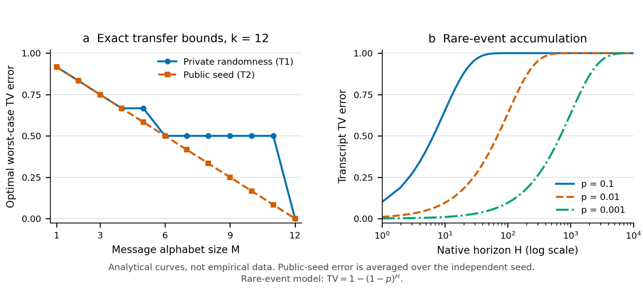
For $k=3,M=2$, private error is $1/2$ and public-seed error is $1/3$. At tolerance $0.4$, the private problem needs three messages while the public problem needs two. The improvement consumes a different coordination resource. If the source may be chosen after observing the seed, or if the error guarantee must hold for every seed separately, this averaged advantage does not follow.

For several local-summary fibres, the decoder can reuse message labels and use the known summary to choose the relevant code. Worst-fibre message requirements are the maxima of the displayed expressions. A finite common seed can provide each fibre’s uniform cyclic choice, for example through a uniform variable on a common multiple of the fibre sizes. This may be expensive; it is an existence construction, not a claim of optimal total physical cost. At $\epsilon=0$, the required message count reduces to the inherited exact fibre count. At $\epsilon=1$, a single message suffices under the convention that the alphabet is nonempty.

8.4 Philosophical significance and limits of the transfer result

The result gives concrete content to the claim that some relational organisation must be retained. It specifies what the recipient must reproduce, which local information is protected, and how a coordination resource changes the necessary communication. It also shows why a count of visible messages cannot by itself measure how much organisation is physically involved. The decoder, seed, installed state and future native dynamics all participate.

Shared randomness changes the distribution of errors without creating information about a source that is independent of it. Its role is coordinated selection of a code. The exact-state limit remains intact: an exact code must preserve every relevant state distinction. Approximate transfer permits a controlled probability of losing the distinction, and that probability is visible under a common revealing continuation.

These theorems do not show that a live exchange is necessary to acquire the organisation. A static lawful installation of the same retained state can meet the same continuation target. They also do not establish a phenomenal equivalence between implementations with different physical contracts. Their contribution is a precise transfer frontier inside a nominated model, suitable for testing how much of a developmental effect resides in accessible retained state.

8.5 Exact finite setting

Let a closed finite state space have $N$ states and common normalized joint instruments $K_{u,o,c}$. The recorded symbol includes the event cost $c$, so budget and deadline tests are functions of the same retained transcript. All actions used here must be admitted throughout the nominated domain. A finite operating grammar may be compiled into the state only when the resulting common-experiment construction satisfies these hypotheses; no extension to arbitrary state-dependent action permissions is assumed. A mathematically added failure action does not supply a physically unavailable intervention.

Write $a=(u,o,c)$ and $K_w=K_{a_1}\cdots K_{a_h}$. Define

$$W=\operatorname{span}\{K_w\mathbf 1:w\text{ is a finite admitted word}\},\qquad r=\dim W.$$

In the ordinary common-action setting, $W$ is obtained by closure from $\mathbf1$ under left multiplication by all $K_a$. A word-column basis can be chosen with lengths at most $r-1\le N-1$: until stability, every refinement increases dimension by at least one. Equality of an iterate with its successor implies permanent invariance. This construction is inherited from the monograph.

A diagnostic is an admitted finite causal protocol with a retained terminal score in $[0,1]$. Its score vector $f\in[0,1]^N$ gives the expected score from each actual starting state. Every such vector belongs to $W$: expand its finite policy tree into leaves; each leaf contributes its common policy randomization factor times its bounded terminal score times a word column. State-dependent oracle access is excluded. A randomized protocol is handled by the same expansion or by linearity.

Two different known machines can be compared by their block-diagonal disjoint union, including the machine label in the mathematical state. The label is not thereby revealed to the experimenter. The same policy and record grammar must apply to both blocks. Initial preparation distributions $\mu,\nu$ may occupy different blocks.

8.6 Diagnostic completeness, including its exact converse

Choose admitted diagnostics $f_1,\ldots,f_m$, and put

$$T=\operatorname{span}\{\mathbf1,f_1,\ldots,f_m\}\subseteq W.$$

Theorem D1. The following are equivalent:

1. $T=W$.

2. For every pair of distributions $\mu,\nu$ in the full probability simplex on the nominated state carrier, equality of all selected diagnostic means $\mu f_j=\nu f_j$ implies equality of every admitted finite adaptive transcript law.

Consequently at least $r-1$ scalar diagnostics are necessary for this universal preparation-distribution guarantee, and $r-1$ suffice when a basis of physically admitted word tests is available. This is a rank requirement, not a claim that $r-1$ different training tasks are intrinsically necessary for a conscious vessel.

Proof. If $T=W$, equality of the selected means and normalization implies $(\mu-\nu)v=0$ for all $v\in W$. Every event probability in every finite adaptive experiment is such a vector, so all event probabilities agree.

Conversely suppose $T\subsetneq W$. There is a real row $d$ annihilating $T$ but not all of $W$: choose a vector in $W\setminus T$ and separate it from $T$ by finite-dimensional linear algebra. Because $\mathbf1\in T$, $d\mathbf1=0$. Let $p$ be the strictly positive uniform probability row and choose $s>0$ so small that $p\pm sd$ are nonnegative. Define $\mu=p+sd$, $\nu=p-sd$. They are probability distributions, agree on every $f_j$, and differ on some $v\in W$. Since word columns span $W$, at least one admitted word probability differs. Its open-loop word test is a finite experiment distinguishing the preparations. This proves the converse. Finally, $\dim T\le m+1$, while a word basis containing $\mathbf1$ supplies $r-1$ nonconstant diagnostic columns. $\square$

Preparation-domain qualification. The converse quantifies over the full mathematical probability simplex. A physical application needs access to that preparation family, or a separate completeness analysis restricted to its lawful preparations. If only a smaller family is available, $T=W$ remains sufficient, but the stated necessity and the $r-1$ lower bound need not hold. The proof does not manufacture the required physical preparation operations.

Actual-state caution. The converse is false if “every preparation distribution” is replaced by “every actual state.” In a three-state device that natively reports its current state, $W=\mathbb R^3$. The single score vector $f=(0,1/2,1)^\top$ distinguishes all three actual states. Nevertheless the mixture $(1/2,0,1/2)$ and the state preparation $(0,1,0)$ have the same score. Their native report laws differ. Thus a scalar can injectively label finitely many actual predictive classes while remaining insufficient for arbitrary mixtures. Exact injectivity is also a poor robustness guarantee if nearby scores have small separation.

Developmental interpretation. It is not necessary to claim that every capability panel is strictly weaker than the native predictive object. A deliberately diagnostic panel can identify its predictive classes under a known finite model. Ordinary performance means generally have no such completeness guarantee. A mean improvement remains different from a change in the full native organisation, and neither score completeness nor a fitted finite model establishes the physical native contract.

8.7 Uniform adaptive transfer from a conditioned diagnostic basis

Assume $B=[\mathbf1,f_1,\ldots,f_{r-1}]$ is an $N\times r$ basis matrix for $W$. Choose any $r$ row indices $I$ such that the square submatrix $A=B_I$ is invertible. Let

$$p=(\mu-\nu)B=(0,\Delta_1,\ldots,\Delta_{r-1}).$$

Define $d_{\rm ad}(\mu,\nu)$ to be the supremum of TV distances over all common admitted finite adaptive transcript experiments; the supremum ranges over arbitrary finite horizons, not an unbounded physical experiment run for free.

Theorem D2. Under the exact fixed-model assumptions above,

$$d_{\rm ad}(\mu,\nu) \le \min\left\{1,\frac12\|pA^{-1}\|_1\right\} \le \min\left\{1,\frac12\sum_{j=1}^{r-1}|\Delta_j|\,\|(A^{-1})_{j,:}\|_1\right\}. \tag{D2}$$

The same bound controls every admitted bounded capability-score difference, including a cost-limited success score. In particular, if valid simultaneous uncertainty bounds give $|\Delta_j|\le\eta_j$, replacing each $|\Delta_j|$ by $\eta_j$ gives a uniform certificate. Different nonsingular row selections or diagnostic bases can give different bounds; one may minimize over the choices actually constructed.

Proof. For any fixed experiment and any event in its finite transcript space, let $v\in[0,1]^N$ be its conditional event-probability vector. By the policy-tree expansion $v\in W$. Therefore $v=B\alpha$ for a unique $\alpha$, and $\alpha=A^{-1}v_I$. The event-probability difference is

$$(\mu-\nu)v=pA^{-1}v_I.$$

Put $w=pA^{-1}$. Since the first column of $A$ is $\mathbf1$, $A^{-1}\mathbf1=e_0$ and hence $w\mathbf1=p_0=0$. For any zero-sum row $w$ and any $t\in[0,1]^r$,

$$|wt|\le\frac12\|w\|_1,$$

because the total positive and negative masses of $w$ each equal half its $\ell_1$ norm. Taking the supremum over transcript events gives the TV bound for that experiment, and the constant does not depend on the horizon or policy. Supremizing over finite experiments proves the first inequality. Rows of $A^{-1}$ are indexed from zero, with row zero corresponding to the constant diagnostic. The second inequality follows by the triangle inequality and $p_0=0$. An expected $[0,1]$-score has exactly the same bounded-vector argument. $\square$

What is doing the work. This does not infer an unknown physical kernel from a small diagnostic panel. The exact finite family supplies $W$, a complete diagnostic basis and its conditioning. The panel then identifies the preparation’s predictions within that family. Model misspecification or transition-row estimation errors require separate bounds. Paper 2’s finite-call error budget can transport a fixed-horizon claim through such errors; its accumulating error cannot simply be omitted to obtain an all-future physical certificate.

The claim concerns trace laws. It does not supply strong actual-successor congruence, an economical decoder, a readable internal-state label, A1 admission, a new native actuator, or A2 validation. It is stronger than a finite panel of unrelated task scores precisely because diagnostic completeness is proved relative to the specified model.

Optional tighter finite optimization. Given exact $p$,

$$\tau_B(p)=\max_{\alpha:0\le B\alpha\le\mathbf1}p\alpha$$

is a finite linear-programming upper bound on $d_{\rm ad}$. The feasible set is symmetric under $\alpha\mapsto e_0-\alpha$, so the maximum also controls the absolute difference. It relaxes operationally implementable event vectors to all bounded vectors in $W$, so equality with the operational metric is not asserted. The matrix $B$ has full column rank; hence the bounded image constraints imply a bounded feasible set. This is a convenient dual/observability bound, not an algorithm claiming exact evaluation of all-future adaptive TV.

8.8 A sharp obstruction to dimension-only approximate certificates

Proposition D3. No universal function $g_N(\eta)\to0$ as $\eta\to0$, depending only on state dimension $N$, can bound all-future adaptive TV from agreement to accuracy $\eta$ on an arbitrary exact word basis, even when the combined dimension is two and there is no feedback or action choice.

Proof and sharp example. Machine $M_0$ has one state and always emits zero. Machine $M_p$ has one state and independently emits one with probability $p\in(0,1)$ each tick. Every tick costs one. Their combined observable space has dimension two with basis matrix

$$B=A=\begin{pmatrix}1&0\\1&p\end{pmatrix}, \qquad A^{-1}=\begin{pmatrix}1&0\\-1/p&1/p\end{pmatrix}.$$

The only nonconstant basis test is “one on the next tick,” whose probability gap is $p$. After $H$ ticks the all-zero word has probability one under $M_0$ and $(1-p)^H$ under $M_p$. Thus

$$\operatorname{TV}(P_0^{H},P_p^{H})=1-(1-p)^H, \qquad d_{\rm ad}=1.$$

The bound in D2 is exactly one: its conditioning factor is $1/p$. Letting $p\downarrow0$ disproves every dimension-only bound tending to zero. $\square$

This also shows why a finite exact equivalence theorem cannot silently become a finite empirical proof of indefinite transfer fidelity. A rare but persistent failure mechanism can remain almost invisible to a short panel and dominate a sufficiently long continuation.

Finite observation lower bound. Suppose an experimenter must discriminate $M_0$ from $M_p$, observing at most $L$ ticks in total, with arbitrary stopping and private randomization. Their complete observation-law TV is at most $1-(1-p)^L$. Therefore any binary decision rule has type-I plus type-II error at least $(1-p)^L$. To make both errors at most $\alpha<1/2$, a necessary condition is

$$L\ge \frac{\log(2\alpha)}{\log(1-p)}.$$

Proof. Couple the processes until the first one emitted by $M_p$. Over $L$ possible draws the probability of no such emission is $(1-p)^L$; an earlier stop cannot improve the full observation-law TV. Under any binary test with acceptance event $E$, the sum of errors is $1-P_p(E)+P_0(E)\ge1-\operatorname{TV}(P_p,P_0)$. The logarithmic inequality follows. $\square$

No bound depending only on finite state count can guarantee a finite uniform empirical certification budget as $p$ is allowed to approach zero. A justified separation or conditioning bound, or a finite horizon, is substantive additional information.

Open figure at full resolutionFigure PDF