8 Executed finite calculations and matched controls
8.1 Fixed preparations and numerical methods
Use the three-node path, with
Three real unit inputs are uniform , contrast , and one port . From , run to and retain 1001 samples. Each control fixes with identical input and initial amplitude. The source has six real amplitude coordinates and two memories, retaining collective and repeated modes. Three integrated coordinates record dissipation, supplied work and tilted loss.
DOP853 uses relative/absolute tolerances , tightened to . A source-derived step cap is
Here includes the second initial state. Equation (13) bounds the largest amplitude scale; eight-step resolution is numerical, not an error enclosure. Independent real-gradient RK4 compares all eight states and three ledgers with 50,000 steps of size . Direct eight-real stationary roots with the complete Hessian Jacobian are compared to a three-real Lambert- root. For real input, real makes share a complex phase. Root tolerance is .
Table 1. Stationary matched controls. Contrast is the norm of the amplitude after subtracting the mean. Edge difference is the absolute difference of the two weights.
| Input | Fixed contrast | Adaptive contrast | Memory norm | Edge difference | Stationary power |
|---|---|---|---|---|---|
| Uniform | 0.0000000 | 0.0000000 | 0.0000000 | 0.0000000 | 0.3333333 |
| Contrast | 0.5323971 | 0.5605998 | 0.1032862 | 0.0000000 | 0.3333333 |
| One port | 0.3869536 | 0.4040033 | 0.0746299 | 0.0591111 | 0.3333333 |
Table 2. Complete equilibrium stability. The final column evaluates the parameter bound independently of the computed eigenvalues.
| Input | |||
|---|---|---|---|
| Uniform | 0.4000000 | −0.2400000 | 0.00393374 |
| Contrast | 0.4000000 | −0.2400000 | 0.00393374 |
| One port | 0.4000000 | −0.2400000 | 0.00393374 |
The original unconstrained-step run failed one frozen criterion: sampled uniform contrast exceeded , with coarse/tight difference . The exact control identifies numerical symmetry error. The original code and results remain available. The cap (48) was frozen before refined outcomes, applied to every source solve, with original thresholds unchanged. The refined run passes 55 frozen criteria. This is post-result refinement, not untouched validation.
8.2 Stationary organization, power and stability
The contrast norm is , memory norm is , and edge heterogeneity is . Tables and figures use the retained outputs at displayed precision. The symmetric memories both equal . One-port memories are , with edge difference . Stored adaptive energies are in input order; fixed-carrier energies are . Equal stationary power coexists with different organization and energy. The preparations impose the contrast mode.
A 60-decimal independent scalar bisection of (32) on reproduces (33) without SciPy or Lambert-. This checks an inspected prediction rather than producing a new holdout or interval certificate. The ledgers separately check
and
A second one-port initial state with real amplitude , imaginary amplitude , and memory gives terminal error .
8.3 Conditional ordering and full response
Integrate conditional propagators and affine columns to on the dense source history. The commutator quadrature samples 401 times. The symmetric contrast factorization gap is about versus for one port. Interaction-picture and affine reconstruction errors remain near numerical precision. Omitting the affine term produces amplitude errors of about , respectively. Quadrature estimates the integral but is not a rigorous upper enclosure.
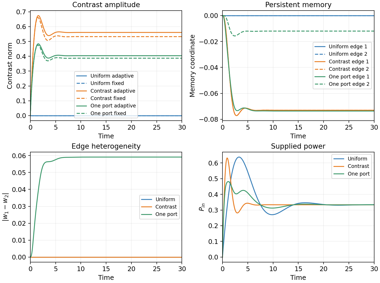
Figure 1. Identically driven adaptive and fixed-carrier controls. The uniform preparation sustains only the collective mode. The symmetric contrast preparation adapts with equal edge memories. One port retains unequal memories. All powers approach under the stated port contract.
At one-port equilibrium compare a real first-coordinate impulse at time , frequency transfer at , and static and Jacobian central differences with step . Nonzero full/clamped gaps distinguish the response contracts. confirms failed complex alignment of the complete tangent.
8.4 Reproducibility and evidence scope
The archive includes frozen specifications, implementations, failed initial outputs, refined results, 13 trajectory arrays, independent scalar check, generated assets, claim map and reproduction runner. Its checker fixes discrete definitions and thresholds, normalizes line endings, and compares generated tables with their own outputs at printed precision. Numerical residuals are judged by scientific criteria rather than incidental digits. The initial failure and step-cap refinement are distinguishable. With the listed dependencies, run python regression_checks.py and python run_all.py --output ../my-new-empty-verification-run in the extracted package.
Table 3. Maximum diagnostics over preparations. The table reports maxima over the preparations except separately specified one-port diagnostics. Upper criteria are strict.
| Diagnostic | Observed | Criterion: less than |
|---|---|---|
| Equilibrium residual | 4.714e-16 | 1.0e-09 |
| Direct/reduced root difference | 3.097e-15 | 1.0e-08 |
| Terminal equilibrium error | 7.035e-11 | 2.0e-07 |
| Coarse/tight trajectory difference | 1.137e-13 | 2.0e-07 |
| Physical energy ledger | 1.066e-13 | 2.0e-07 |
| Tilted loss ledger | 3.331e-15 | 2.0e-07 |
| Collective-mode formula | 9.155e-16 | 1.0e-09 |
| Independent real-gradient RK4 | 2.792e-12 | 2.0e-07 |
| Second initial-state terminal error | 4.231e-11 | 2.0e-07 |
Table 4. Response and conditional history. Transfer gaps use operator norm. The impulse uses the first real-coordinate probe. Quadrature is a numerical diagnostic.
| Quantity | Value |
|---|---|
| Full/clamped impulse gap | 1.810309e-02 |
| Full/clamped static transfer gap | 4.678222e-02 |
| Full/clamped frequency transfer gap | 4.440963e-02 |
| Full Jacobian finite difference | 1.580285e-11 |
| Static probe finite difference | 1.825302e-11 |
| Contrast factorization gap | 3.257883e-15 |
| Contrast interaction error | 5.651507e-15 |
| Contrast affine error | 2.830524e-16 |
| Contrast commutator quadrature | 0.000000e+00 |
| One port factorization gap | 4.926845e-04 |
| One port interaction error | 5.154423e-15 |
| One port affine error | 5.926969e-16 |
| One port commutator quadrature | 2.093538e-01 |
The retained numerical environment was Python 3.12.14, NumPy 2.3.5, SciPy 1.18.1 on Windows. RK4, direct/reduced roots, and Decimal bisection test different formulations. Analytic proofs, exact negative curvature and the rational stability margin establish their stated mathematical claims. Floating trajectories, eigenvalues and quadrature are not directed interval certificates. Physical validation still requires calibrated actuator and paired probes.
9 Consequences and focused extensions
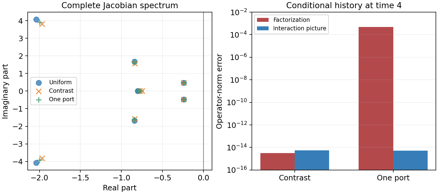
Figure 2. Complete stability and response. Left: all eight equilibrium Jacobian eigenvalues for each preparation, retaining multiplicities. Right: transient conditional factorization and interaction-picture errors for the two nonuniform preparations. The one-port transient relaxes to a constant carrier, but free/clamped transfer differences persist at equilibrium.
A sharp scalar curvature bound supplies an all-input sufficient attraction regime. The complete Hessian proves local stability without requiring global joint convexity. Symmetric contrast turns the stationary reduction into an exact gain law, and continuing work pays for sustained organization. Conditional phase and attenuation share a carrier; the free-memory probe retains a causal kernel. A common mean or equal power misses that distinction. The direct experiment would calibrate the energy effort, quadrature ports and memory, then compare static and phase-sensitive frequency response with and without clamping.
Time-varying drive needs a different Lyapunov argument, finite reservoirs require a supply state and depletion, and parameters outside the strict sufficient regime need separate stability analysis. Continuum limits and cross-domain microscopic identification remain open. Within the declared finite constant-input class, the construction proves attraction in its regime, quantifies gains beyond imposed preparation, and separates conditional linkage from complete response.
References
- Jeremy Rodgers. The Canonical Spectral-Curvature Field: A Unified Operator Origin for Coherence, Dissipation, and Spectral Budgets. 2026a, Zenodo preprint. DOI.
- Jeremy Rodgers. Adaptive Spectral Carriers: Time Ordering, Reciprocal Memory, and Linked Coherent–Dissipative Response. 2026b, Zenodo preprint. DOI.
- Jeremy Rodgers. Source Readout Non-Equivalence: Descent and Equivariant Reconstruction Obstructions. 2026c, Zenodo preprint. DOI.
- Jeremy Rodgers. Observable Quotients and Exact Projected Dynamics: Closure, Memory, Minimal Dynamical Completion, and Effective Field Operators. 2026d, Zenodo preprint. DOI.
- Arjan van der Schaft and D. Jeltsema. Port-Hamiltonian Systems Theory: An Introductory Overview. Vol. 1 of Foundations and Trends in Systems and Control, nos. 2–3. Now Publishers, 2014. DOI.
- Robert M. Corless, Gaston H. Gonnet, D. E. G. Hare, David J. Jeffrey, and Donald E. Knuth. On the Lambert W function. Advances in Computational Mathematics 5:329–359, 1996. DOI.
- J. P. LaSalle. The Stability of Dynamical Systems. Vol. 25, CBMS-NSF Regional Conference Series in Applied Mathematics. SIAM, 1976. DOI.
Published source: Sustained Adaptive Spectral States: Global Attraction, Nonlinear Gain, and Linked Coherent–Dissipative Response. Read the original PDF alongside the web treatment.