# Sustained Adaptive Spectral States: Global Attraction, Nonlinear Gain, and Linked Coherent–Dissipative Response
Global Attraction, Nonlinear Gain, and Linked Coherent–Dissipative Response
Jeremy Rodgers · 2026-11-03
DOI: https://doi.org/10.5281/zenodo.23927855
## The power that sustains an adaptive state
## 1 From relaxing carriers to sustained adaptive states
External input can maintain a carrier that would otherwise relax. In the fixed-carrier CSCF [Rodgers 2026a], one positive operator links coherence and dissipation. Reciprocal adaptation [Rodgers 2026b] gives this operator a memory state; positive unforced amplitudes decay and memory returns to zero. Sustaining a nonzero state requires work and an explicit account of what the actuator imposes.
Prescribe a constant complex rate input. The preparation determines spatial mode and phase, while reciprocal feedback determines amplitude, memory, stiffness and response. The problem is to identify an all-input attraction regime, measure the departure from an identically driven fixed carrier, and recover which linked responses survive adaptation. The amplitude or instantaneous spectrum alone need not predict a later response after memory changes. The causal kernel below makes the missing source information explicit [Rodgers 2026c,d]. Stationary elimination determines equilibrium without replacing memory dynamics, and a three-node path provides exact collective and contrast controls, nonlinear gain and an equal-power comparison. No shared microscopic origin of earlier atomic, image or Kerr profiles follows.
## 2 Source state, actuator and physical energy
### 2.1 Constitutive equations and units
For $z\in\mathbb C^n,m\in\mathbb R^p$ and real incidence vectors $b_e$, take
$$
B_e=b_e b_e^\top,\qquad L=\sum_{e=1}^p B_e,\qquad K(m)=\mu I+\sum_{e=1}^p e^{m_e}B_e,\quad\mu>0.\tag{1}
$$
Edge baselines are normalized to one; positive $k_e$ can instead be absorbed in $\sqrt{k_e}b_e$, with $L$ and bounds using those same scaled vectors. The metric is fixed and Euclidean, and norms are Euclidean and induced unless specified. $K\ge\mu I$, including on the collective subspace.
$$
F(z,m)=\tfrac12 z^*K(m)z+\tfrac\kappa2|m|^2,\qquad \kappa>0,\tag{2}
$$
$$
(F_m)_e=\kappa m_e+\tfrac12 e^{m_e}|b_e^\top z|^2.\tag{3}
$$
Let $c=\gamma+i\alpha$, with $\gamma,\alpha,\eta>0$. The dynamics are
$$
\dot z=-cK(m)z+f,\qquad \dot m=-\eta F_m(z,m),\quad f\in\mathbb C^n\text{ constant}.\tag{4}
$$
No target profile adjusts $f$. Positive $\eta$ couples memory to the same energy that produces the amplitude effort. This reciprocity is constitutive. In amplitude units $A$ and energy units $E$, $m,b_e$ are dimensionless before baseline absorption, $K,\mu$ and unnormalized edge coefficients have units $E/A^2$, $\kappa$ has units $E$, $f$ has units $A/\mathrm s$, $\gamma,\alpha$ have units $A^2/(E\,\mathrm s)$, and $\eta$ has units $1/(E\,\mathrm s)$. Scales $A_0,E_0,t_0$ normalize the equations with $\tilde f=t_0f/A_0$. Joint-state norms below use these normalized coordinates; mixing units would make rate bounds arbitrary.
### 2.2 The effort–flow input contract
For $q=(\Re z,\Im z)^\top$,
$$
K_R=\operatorname{diag}(K,K),\quad J=\begin{pmatrix}0&-I\\ I&0\end{pmatrix},\quad G=\gamma I+\alpha J,\quad f_R=(\Re f,\Im f)^\top.\tag{5}
$$
Each quadrature port imposes a flow $f_R$ with energy-conjugate effort $y=K_Rq$. Its supplied power is
$$
P_{\rm in}=y^\top f_R=\Re[(Kz)^*f].\tag{6}
$$
In dissipative port-Hamiltonian form [van der Schaft and Jeltsema 2014], $x=(q,m)$ satisfies
$$
\dot x=(\mathcal J-\mathcal R)\nabla F+\mathcal B f_R,\quad \mathcal J=\operatorname{diag}(-\alpha J,0),\quad
\mathcal R=\operatorname{diag}(\gamma I,\eta I),\quad \mathcal B=\begin{pmatrix}I\\0\end{pmatrix},\quad y=\mathcal B^\top\nabla F.\tag{7}
$$
The skew part contributes zero to $\dot F$; direct differentiation gives
$$
\dot F=-\gamma\|Kz\|^2-\eta\|F_m\|^2+P_{\rm in}.\tag{8}
$$
At steady state external and internal amplitude flows cancel while input power covers dissipation. The supply is outside the modeled state, not a modeled finite reservoir; arbitrary initial data can give negative power, so the ideal actuator must absorb returned energy. A laboratory envelope requires an independent clock and phase reference, calibrated quadrature actuator, and validation of the stored energy and conjugate effort. An arbitrary optical pump need not realize this contract.
## 3 Global solutions and the stationary reduction
### 3.1 A mathematical tilt distinct from stored energy
Set $\ell=f/c$, in units $E/A$. For constant input use
$$
V(z,m)=F(z,m)-\Re(\ell^*z).\tag{9}
$$
Because $f_R=G\ell_R$,
$$
\dot q=-GV_q,\quad \dot m=-\eta V_m,\quad\dot V=-\gamma\|Kz-\ell\|^2-\eta\|F_m\|^2.\tag{10}
$$
The tilt exists for any constant input; it does not select that input or replace the physical work balance (8).
**Proposition 3.1 (Global forward existence).** For all positive parameters above, finite incidence networks, constant $f$ and finite initial data, (4) has a unique bounded forward solution.
**Proof.** Young's inequality gives
$$
V\ge\tfrac\mu4\|z\|^2+\tfrac\kappa2|m|^2-\|\ell\|^2/\mu.\tag{11}
$$
The smooth vector field is locally Lipschitz; (10) keeps it in a compact sublevel. Continuation there excludes finite escape and local uniqueness gives global uniqueness.
The upper right Dini derivative satisfies $D^+\|z\|\le-\gamma\mu\|z\|+\|f\|$, also at $z=0$. Thus
$$
\|z(t)\|\le e^{-\gamma\mu t}\|z(0)\|+\frac{\|f\|}{\gamma\mu}(1-e^{-\gamma\mu t}).\tag{12}
$$
Also $\dot m_e<0$ for $m_e>0$ and $\dot m_e\le0$ at zero:
$$
m_e(t)\le\max\{0,m_e(0)\},\quad K(t)\le\mu I+e^{M_0}L,\qquad M_0=\max\{0,m_1(0),\ldots,m_p(0)\}.\tag{13}
$$
### 3.2 Eliminating memory at stationarity
For fixed $z$,
$$
\partial_{m_e}^2F=\kappa+\tfrac12e^{m_e}|b_e^\top z|^2\ge\kappa.\tag{14}
$$
The coercive strictly convex memory slices have unique minimizers $m_e=-s_e$:
$$
s_e e^{s_e}=\frac{|b_e^\top z|^2}{2\kappa},\qquad s_e=W_0\left(\frac{|b_e^\top z|^2}{2\kappa}\right)\ge0.\tag{15}
$$
Here $W_0$ is the nonnegative real Lambert branch [Corless et al. 1996]. Edge amplitude energy is $\kappa s_e$, and memory energy $\kappa s_e^2/2$. Hence
$$
V_{\rm eff}(z)=\tfrac\mu2\|z\|^2+\sum_e\kappa(s_e+s_e^2/2)-\Re(\ell^*z).\tag{16}
$$
Positive memory second derivatives justify implicit differentiation. The real-coordinate envelope gradient is the realification of $K(m(z))z-\ell$, so critical points correspond exactly to equilibria once memory is restored by (15). Substituting $-s(z(t))$ dynamically would remove a state and change transients and response.
### 3.3 Why global joint convexity is unavailable
For the three-node path $b_1=(1,-1,0)^\top,b_2=(0,1,-1)^\top$, $\mu=2/5,\kappa=1,z=(3,0,-3)^\top$ real and $m=0$, the real-amplitude/memory Hessian has
$$
K=\mu I+L,\qquad B=3[b_1,b_2],\qquad H_m=\tfrac{11}2I.\tag{17}
$$
Its Schur complement is $\mu I-(7/11)L$. For $\xi=(1,0,-1)^\top$ and $\nu=(-6/11,-6/11)^\top$ with imaginary perturbation zero the joint quadratic form is $-26/55$. The tilt leaves the Hessian unchanged. This exact obstruction motivates stationary reduction followed by a complete local stability analysis; it supplies no global Euclidean contraction theorem.
## Global attraction and nonlinear gain
## 4 Sharp curvature and global attraction
**Lemma 4.1 (Reduced edge curvature).** For $d\in\mathbb C,r=|d|,s=W_0(r^2/(2\kappa)),w=e^{-s}$, the two real Hessian eigenvalues of $\kappa(s+s^2/2)$ are
$$
\lambda_{\rm tan}=w,\qquad\lambda_{\rm rad}=w\frac{1-s}{1+s}.\tag{18}
$$
Both are one at the origin by continuity. The sharp scalar lower bound is $-\chi$, where
$$
\chi=(2-\sqrt3)e^{-\sqrt3}=0.0474058943568\ldots.\tag{19}
$$
**Proof.** From $se^s=r^2/(2\kappa)$, $ds/dr=2s/[r(1+s)]$ for $r>0$. Differentiate the edge gradient $wd$: its tangential eigenvalue is $w$ and its radial eigenvalue $w+r\,dw/dr$ is (18). For $s\le1$ both are nonnegative; for $s>1$,
$$
\frac d{ds}\left[e^{-s}\frac{s-1}{s+1}\right]=e^{-s}\frac{3-s^2}{(s+1)^2}.\tag{20}
$$
The magnitude peaks at $s=\sqrt3$ with value $\chi$. Every $s\ge0$ is attained for some $r$, proving scalar sharpness without assuming simultaneous worst directions on all graph edges.
Pull back the edge Hessians through $z\mapsto b_e^\top z$:
$$
\nabla^2 V_{\rm eff}\ge\mu I-\chi L_R\ge\delta I,\qquad L_R=\operatorname{diag}(L,L),\quad\delta=\mu-\chi\|L\|.\tag{21}
$$
The spectral norm includes all multiplicities and collective modes.
**Theorem 4.2 (Unique sustained state and global attraction).** Under the positivity hypotheses and $\delta>0$, every constant complex $f$ has one globally asymptotically stable equilibrium, with $\|z_*\|\le\|\ell\|/\mu$, $m_*\le0$.
**Proof.** The coercive $V_{\rm eff}$ is strongly convex by (21), so its unique critical point is the unique minimizer $z_*$. The strictly convex memory slices restore $m_*$. At equilibrium $K(m_*)z_*=\ell$, giving the norm bound, and (15) gives the memory sign.
Along any bounded trajectory $V$ converges to a finite limit. Write $g=\gamma\|Kz-\ell\|^2+\eta\|F_m\|^2$. An omega-limit point with $g>0$ would have a ball where $g\ge\epsilon>0$. Bounded speed on a compact neighborhood forces a positive residence time in that ball after each visit to a smaller concentric ball, unless the trajectory never leaves, in which case $V\to-\infty$. Infinitely many disjoint residence intervals likewise force unbounded loss. Therefore all omega-limit points have $g=0$; compactness and the unique equilibrium then imply convergence of the entire trajectory.
Moreover $V(z,m)\ge V_{\rm eff}(z)\ge V_{\rm eff}(z_*)=V(z_*,m_*)$, with equality only there. On a small sphere around the equilibrium the excess has a positive minimum. Initial states in a smaller sublevel cannot cross it by (10), proving Lyapunov stability. This direct finite-dimensional invariance argument [LaSalle 1976] gives global convergence, without a uniform global exponential or intertrajectory contraction estimate. Failure of the strict sufficient condition alone establishes neither instability nor multistability.
## 5 Complete local stability and a parameter bound
At equilibrium $q_*=(\Re z_*,\Im z_*)^\top$, set
$$
H=\begin{pmatrix}K_R&B\\B^\top&H_m\end{pmatrix},\quad B_{\cdot e}=e^{m_{*,e}}\operatorname{diag}(B_e,B_e)q_*,\quad
H_m=\operatorname{diag}\big(\kappa+\tfrac12 e^{m_{*,e}}|b_e^\top z_*|^2\big).\tag{22}
$$
Differentiating stationary memory gives $dm/dq=-H_m^{-1}B^\top$, hence
$$
S=K_R-BH_m^{-1}B^\top=\nabla^2 V_{\rm eff}(z_*)\ge\delta I.\tag{23}
$$
Consequently $H>0$. The constant-mobility Jacobian is
$$
A_{\rm full}=-DH,\qquad D=\operatorname{diag}(G,\eta I),\qquad\tfrac12(D+D^\top)=\operatorname{diag}(\gamma I,\eta I).\tag{24}
$$
Partial amplitude curvature alone cannot establish this joint-state result.
**Proposition 5.1 (Linear rate and nonlinear local stability).** With $\sigma=\min\{\gamma,\eta\}$, define
$$
\theta_0=\frac{\|\ell\|\sqrt{\sum_e\|b_e\|^4}}{\kappa\mu},\qquad h_0=\frac{\min\{\delta,\kappa\}}{(1+\theta_0)^2}>0.\tag{25}
$$
Then $H\ge h_0 I$, and for $\|v\|_H=(v^\top Hv)^{1/2}$,
$$
\|v(t)\|_H\le e^{-\sigma h_0 t}\|v(0)\|_H,\qquad\max_{\lambda\in\operatorname{spec}(A_{\rm full})}\Re\lambda\le-\sigma h_0.\tag{26}
$$
Every positive rate strictly below $\sigma h_0$ holds for nonlinear evolution in a sufficiently small neighborhood in the equilibrium Hessian norm.
**Proof.** Since $m_*\le0$, $\|B_{\cdot e}\|\le\|b_e\|^2\|z_*\|$, hence $\|H_m^{-1}B^\top\|\le\kappa^{-1}\|B\|\le\theta_0$. Completing the square gives
$$
(\xi,\nu)^\top H(\xi,\nu)=\xi^\top S\xi+(\nu+H_m^{-1}B^\top\xi)^\top H_m(\nu+H_m^{-1}B^\top\xi).\tag{27}
$$
The inverse shear has norm at most $1+\theta_0$. Combine (23) and $H_m\ge\kappa I$ to get $H\ge h_0I$. For $E_v=v^\top Hv/2$, the linearized system gives
$$
\dot E_v=-(Hv)^\top\operatorname{diag}(\gamma I,\eta I)(Hv)\le-\sigma h_0 v^\top Hv=-2\sigma h_0E_v.\tag{28}
$$
Integrate to obtain the norm and spectral bounds. The nonlinear vector field differs by $O(\|v\|^2)$, adding $O(\|v\|^3)$ to $\dot E_v$. Bound it by $2\epsilon E_v$ in a small invariant sublevel for any $0<\epsilon<\sigma h_0$.
The exact linear estimate, local nonlinear rate and numerical eigenvalues remain distinct. A fixed nonzero input fixes phase; at zero input positive $\mu,\kappa$ also remove zero decay rates despite the graph collective mode. For the path, $\|L\|=3,\mu=2/5$. Since $\sqrt3>5/3,\ 2-\sqrt3<1/3$ and the cubic Taylor polynomial for the exponential at $5/3$ exceeds four, $\chi<1/12,\delta>3/20$. With unit input $|c|=\sqrt{9/5}>1$, and $\sqrt{\sum_e\|b_e\|^4}=\sqrt8<3$, giving $\theta_0<15/2,\ h_0>3/1445$, and
$$
\sigma h_0>9/7225.\tag{29}
$$
This is conservative: (25) evaluated numerically gives rate $\sigma h_0\approx0.00393374$, while the complete numerical spectral abscissa is about $-0.24$.
## 6 What the drive imposes and feedback changes
### 6.1 Collective control and symmetric contrast gain
With $b_e^\top\mathbf1=0$, $\bar z=n^{-1}\mathbf1^\top z,\ \bar f=n^{-1}\mathbf1^\top f$ satisfy
$$
\bar z(t)=\frac{\bar f}{c\mu}+\left(\bar z(0)-\frac{\bar f}{c\mu}\right)e^{-c\mu t}.\tag{30}
$$
A matched fixed carrier has the same mean. Uniform input and initial amplitude with zero memory keep all contrasts and memories zero. Thus sustained collective amplitude controls for excitation without adaptive edge organization.
For the path take
$$
v=(1,0,-1)^\top/\sqrt2,\qquad f=av,\quad a>0.\tag{31}
$$
Signed reflection (swap endpoints and reverse sign of amplitude) preserves this preparation. Starting from zero gives the invariant sector $z=uv$ and equal memories. At equilibrium $m_1=m_2=-s$; $Lv=v$ and $|b_e^\top z|^2=|u|^2/2$ imply
$$
\frac{a^2}{|c|^2}=4\kappa s e^s(\mu+e^{-s})^2,\qquad u=\frac{a/c}{\mu+e^{-s}}.\tag{32}
$$
For $a>0$, $s>0$. The right side starts at zero and diverges; its derivative has the sign of $\mu+e^{-s}(1-s)/(1+s)$, positive for $\mu>\chi$ by Lemma 4.1. Thus it specifies exactly one $s$ there. The fixed carrier gives $u_0=(a/c)/(\mu+1)$, and
$$
G=\frac{|u|}{|u_0|}=\frac{\mu+1}{\mu+e^{-s}}>1.\tag{33}
$$
The drive specifies the spatial mode and relative phase. Feedback produces nonzero equal memories, persistent softening and excess amplitude. For the worked parameters $s=0.07303438894\ldots,\ G=1.0529729143\ldots$, about 5.30% gain. This is a fixed-preparation prediction. A one-port input retains mean and contrast, and can sustain unequal memories as shown below, without implying every asymmetric input does.
### 6.2 Equal stationary power and continuing work
At equilibrium $Kz_*=\ell,\ F_m=0$, so
$$
P_*=\Re(\ell^*c\ell)=\gamma\|\ell\|^2=\frac{\gamma\|f\|^2}{\gamma^2+\alpha^2}.\tag{34}
$$
The same identity holds for the fixed carrier. Equal-norm inputs have equal stationary power in this contract while differing in amplitude, memory, energy and response.
**Corollary 6.1 (Work required for sustained organization).** Under Theorem 4.2 with $f\ne0$,
$$
\int_0^T P_{\rm in}(t)\,dt=P_*T+o(T),\qquad P_*>0.\tag{35}
$$
Dissipation has the same leading growth, while stored energy converges.
**Proof.** Full convergence gives $P_{\rm in}\to P_*,F\to F_*$. Split the integral at a time after which the difference in power is below any $\epsilon>0$. The early finite integral divided by $T$ vanishes; the remaining average error is at most $\epsilon$. Integrate (8) and use bounded energy change to transfer the leading term to dissipation.
An unreplenished finite work supply cannot maintain the nonzero state forever. Constant forcing represents powered dissipation rather than autonomous oscillation sustained indefinitely by initial energy.
## The driven carrier keeps two kinds of response
## 7 Conditional linkage and complete feedback response
### 7.1 Affine propagation and time ordering
Clamp or replay $m(t)$. The driven amplitude map is affine:
$$
z(t)=U(t,0)z(0)+\int_0^t U(t,s)f\,ds,\qquad\partial_tU(t,s)=-cK(t)U(t,s),\quad U(s,s)=I.\tag{36}
$$
The homogeneous $U$ depends on the fixed history; it is not the full freely adapting derivative. The affine term is necessary to predict driven amplitude. For $A=cK$,
$$
H(t)=\tfrac12(A+A^*)=\gamma K(t),\quad C(t)=\tfrac1{2i}(A-A^*)=\alpha K(t)=\frac\alpha\gamma H(t).\tag{37}
$$
On any finite interval the carrier is bounded. The linear CSCF symbol may be continued constantly beyond its compact reachable spectral interval to satisfy boundedness. Do not fit the mobility on the same response used to test it.
Let $\dot V_c=-i\alpha KV_c,V_c(0)=I$; it is unitary. With $U=V_cR$, differentiate $V_c^*U$:
$$
\dot R=-\gamma V_c^*KV_cR,\qquad R(0)=I.\tag{38}
$$
For $\dot D_c=-\gamma KD_c,D_c(0)=I$, the gap-free comparison is
$$
\|U(T)-D_c(T)V_c(T)\|\le\gamma\alpha\int_0^T\!\int_0^t\|[K(t),K(s)]\|\,ds\,dt.\tag{39}
$$
Fix $t$ and differentiate $Q_t(s)=[K(t),D_c(s)]$:
$$
\dot Q_t(s)=-\gamma K(s)Q_t(s)-\gamma[K(t),K(s)]D_c(s),\quad Q_t(0)=0.\tag{40}
$$
Contraction gives $\|Q_t(t)\|\le\gamma\int_0^t\|[K(t),K(s)]\|ds$. Now $D_cV_c$ has residual $i\alpha[K,D_c]V_c$ in the $U$ equation. Variation of constants, contraction of $U$ and unitarity give (39). Neither a gap nor eigenvector tracking is needed.
For path weights $w_e=e^{m_e}$,
$$
[K(t),K(s)]=[w_1(t)w_2(s)-w_2(t)w_1(s)][B_1,B_2],\qquad \|[B_1,B_2]\|=\sqrt3.\tag{41}
$$
The symmetric contrast sector has equal moving weights and commutes. A one-port transient need not. The attracting equilibrium gives a constant carrier and exact conditional factorization. Transient noncommutation implies neither persistent motion nor a Floquet result.
### 7.2 Memory kernel and transfer operators
At equilibrium, real amplitude and memory perturbations $\xi,\nu$ obey, with additive real rate probe $r(t)$,
$$
\dot\xi=-GK_R\xi-GB\nu+r(t),\qquad\dot\nu=-\eta B^\top\xi-\eta H_m\nu.\tag{42}
$$
The fixed input has no state derivative. Solve the memory block and substitute:
$$
\dot\xi(t)=-GK_R\xi(t)-GBe^{-\eta H_m t}\nu(0)+r(t)+\eta\int_0^t GBe^{-\eta H_m(t-s)}B^\top\xi(s)\,ds.\tag{43}
$$
Zero initial memory perturbation leaves the kernel. The retained amplitude alone loses predictive information without this memory term. For zero initial perturbations, on the complexification of the real amplitude space, the Laplace-domain transfers are
$$
X_{\rm full}(p)=\left[pI+GK_R-\eta GB(pI+\eta H_m)^{-1}B^\top\right]^{-1},\tag{44}
$$
$$
X_{\rm clamp}(p)=(pI+GK_R)^{-1}.\tag{45}
$$
Under Theorem 4.2 they exist on $\Re p\ge0$. Positivity $H_m\ge\kappa I$ makes the eliminated block invertible, and Proposition 5.1 makes $pI-A_{\rm full}$ invertible. Its amplitude Schur complement is therefore invertible. For the clamp, $G$ commutes with $K_R$, with complex generator eigenvalues $-c\lambda_j(K)$ having negative real parts; the realification adds their conjugates. This covers static response and all real frequencies $p=i\omega$. Elsewhere (44) requires both inverses and makes no assertion at an eliminated memory pole.
At zero frequency, use (23):
$$
X_{\rm full}(0)=S^{-1}G^{-1},\qquad X_{\rm clamp}(0)=K_R^{-1}G^{-1}.\tag{46}
$$
Order matters. Free memory changes even the static susceptibility at identical state and probe. $H$ need not commute with $\operatorname{diag}(J,0)$, so conditional complex-linearity cannot generally represent the complete feedback response.
### 7.3 Observable contract and required resources
Calibrate time and the amplitude metric, independently measure mobilities, access both quadratures with phase sensitivity, and prepare enough independent columns to reconstruct the operator. Subtract the driven affine baseline. Reproduce or clamp memory across columns for conditional probes; a free-memory kick instead tests (43) or (44). Pooled magnitudes, instantaneous spectra and a common mean cannot supply this access. The full state, work record and controlled-memory probe retain different source information.
## The driven tests separate power, organization and response
## 8 Executed finite calculations and matched controls
### 8.1 Fixed preparations and numerical methods
Use the three-node path, with
$$
(\mu,\kappa,\gamma,\alpha,\eta)=(0.4,1,0.6,1.2,0.8).\tag{47}
$$
Three real unit inputs are uniform $(1,1,1)^\top/\sqrt3$, contrast $(1,0,-1)^\top/\sqrt2$, and one port $(1,0,0)^\top$. From $z=m=0$, run to $T=100$ and retain 1001 samples. Each control fixes $K=K(0)$ with identical input and initial amplitude. The source has six real amplitude coordinates and two memories, retaining collective and repeated modes. Three integrated coordinates record dissipation, supplied work and tilted loss.
DOP853 uses relative/absolute tolerances $10^{-10}/10^{-12}$, tightened to $10^{-12}/10^{-14}$. A source-derived step cap is
$$
\Delta t_{\max}=\frac1{8|c|(\mu+e^{M_0}\|L\|)}=0.02507581193\ldots .\tag{48}
$$
Here $M_0=0.1$ includes the second initial state. Equation (13) bounds the largest amplitude scale; eight-step resolution is numerical, not an error enclosure. Independent real-gradient RK4 compares all eight states and three ledgers with 50,000 steps of size $0.002$. Direct eight-real stationary roots with the complete Hessian Jacobian are compared to a three-real Lambert-$W$ root. For real input, real $K$ makes $z_*=c^{-1}K^{-1}f$ share a complex phase. Root tolerance is $10^{-11}$.
**Table 1. Stationary matched controls.** Contrast is the norm of the amplitude after subtracting the mean. Edge difference is the absolute difference of the two weights.
| Input | Fixed contrast | Adaptive contrast | Memory norm | Edge difference | Stationary power |
| --- | ---: | ---: | ---: | ---: | ---: |
| Uniform | 0.0000000 | 0.0000000 | 0.0000000 | 0.0000000 | 0.3333333 |
| Contrast | 0.5323971 | 0.5605998 | 0.1032862 | 0.0000000 | 0.3333333 |
| One port | 0.3869536 | 0.4040033 | 0.0746299 | 0.0591111 | 0.3333333 |
**Table 2. Complete equilibrium stability.** The final column evaluates the parameter bound independently of the computed eigenvalues.
| Input | $\lambda_{\min}(H)$ | $\max\Re\lambda(A_{\rm full})$ | $\sigma h_0$ |
| --- | ---: | ---: | ---: |
| Uniform | 0.4000000 | −0.2400000 | 0.00393374 |
| Contrast | 0.4000000 | −0.2400000 | 0.00393374 |
| One port | 0.4000000 | −0.2400000 | 0.00393374 |
The original unconstrained-step run failed one frozen criterion: sampled uniform contrast $7.35254\times10^{-8}$ exceeded $10^{-9}$, with coarse/tight difference $6.34174\times10^{-8}$. The exact control identifies numerical symmetry error. The original code and results remain available. The cap (48) was frozen before refined outcomes, applied to every source solve, with original thresholds unchanged. The refined run passes 55 frozen criteria. This is post-result refinement, not untouched validation.
### 8.2 Stationary organization, power and stability
The contrast norm is $\|z-\bar z\mathbf1\|$, memory norm is $\|m\|$, and edge heterogeneity is $|e^{m_1}-e^{m_2}|$. Tables and figures use the retained outputs at displayed precision. The symmetric memories both equal $-0.07303439$. One-port memories are $-0.07366282,-0.01197548$, with edge difference $0.05911106$. Stored adaptive energies are $0.69444444,0.21425722,0.35254833$ in input order; fixed-carrier energies are $0.69444444,0.19841270,0.34430439$. Equal stationary power coexists with different organization and energy. The preparations impose the contrast mode.
A 60-decimal independent scalar bisection of (32) on $[0,1]$ reproduces (33) without SciPy or Lambert-$W$. This checks an inspected prediction rather than producing a new holdout or interval certificate. The ledgers separately check
$$
F(t)-F(0)+\int_0^t(\gamma\|Kz\|^2+\eta\|F_m\|^2)ds-\int_0^tP_{\rm in}\,ds
$$
and
$$
V(t)-V(0)+\int_0^t(\gamma\|Kz-\ell\|^2+\eta\|F_m\|^2)ds.
$$
A second one-port initial state with real amplitude $(0.4,-0.2,0.1)$, imaginary amplitude $(0.1,0.3,-0.2)$, and memory $(0.1,-0.15)$ gives terminal error $4.23136\times10^{-11}$.
### 8.3 Conditional ordering and full response
Integrate conditional propagators and affine columns to $T=4$ on the dense source history. The commutator quadrature samples 401 times. The symmetric contrast factorization gap is about $3.26\times10^{-15}$ versus $4.92685\times10^{-4}$ for one port. Interaction-picture and affine reconstruction errors remain near numerical precision. Omitting the affine term produces amplitude errors of about $0.54235,1.33548$, respectively. Quadrature estimates the integral but is not a rigorous upper enclosure.
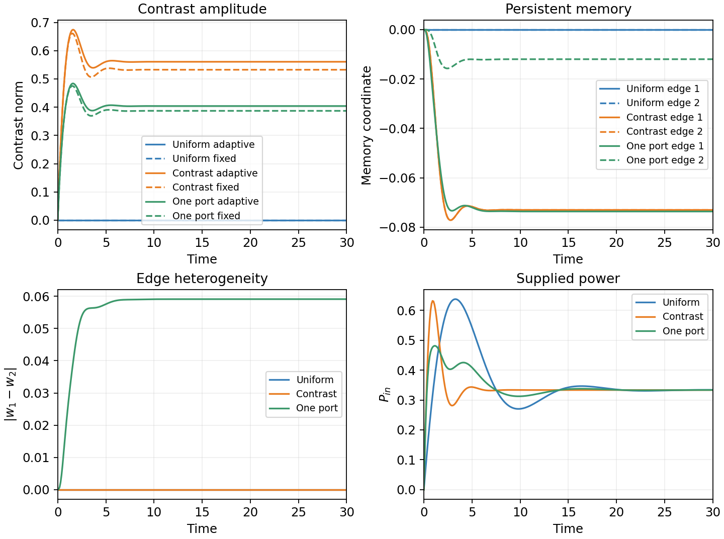
**Figure 1. Identically driven adaptive and fixed-carrier controls.** The uniform preparation sustains only the collective mode. The symmetric contrast preparation adapts with equal edge memories. One port retains unequal memories. All powers approach $1/3$ under the stated port contract.
At one-port equilibrium compare a real first-coordinate impulse at time $2$, frequency transfer at $p=0.5i$, and static and Jacobian central differences with step $10^{-5}$. Nonzero full/clamped gaps distinguish the response contracts. $\|[H,\operatorname{diag}(J,0)]\|=0.53593673$ confirms failed complex alignment of the complete tangent.
### 8.4 Reproducibility and evidence scope
The archive includes frozen specifications, implementations, failed initial outputs, refined results, 13 trajectory arrays, independent scalar check, generated assets, claim map and reproduction runner. Its checker fixes discrete definitions and thresholds, normalizes line endings, and compares generated tables with their own outputs at printed precision. Numerical residuals are judged by scientific criteria rather than incidental digits. The initial failure and step-cap refinement are distinguishable. With the listed dependencies, run `python regression_checks.py` and `python run_all.py --output ../my-new-empty-verification-run` in the extracted package.
**Table 3. Maximum diagnostics over preparations.** The table reports maxima over the preparations except separately specified one-port diagnostics. Upper criteria are strict.
| Diagnostic | Observed | Criterion: less than |
| --- | ---: | ---: |
| Equilibrium residual | 4.714e-16 | 1.0e-09 |
| Direct/reduced root difference | 3.097e-15 | 1.0e-08 |
| Terminal equilibrium error | 7.035e-11 | 2.0e-07 |
| Coarse/tight trajectory difference | 1.137e-13 | 2.0e-07 |
| Physical energy ledger | 1.066e-13 | 2.0e-07 |
| Tilted loss ledger | 3.331e-15 | 2.0e-07 |
| Collective-mode formula | 9.155e-16 | 1.0e-09 |
| Independent real-gradient RK4 | 2.792e-12 | 2.0e-07 |
| Second initial-state terminal error | 4.231e-11 | 2.0e-07 |
**Table 4. Response and conditional history.** Transfer gaps use operator norm. The impulse uses the first real-coordinate probe. Quadrature is a numerical diagnostic.
| Quantity | Value |
| --- | ---: |
| Full/clamped impulse gap | 1.810309e-02 |
| Full/clamped static transfer gap | 4.678222e-02 |
| Full/clamped frequency transfer gap | 4.440963e-02 |
| Full Jacobian finite difference | 1.580285e-11 |
| Static probe finite difference | 1.825302e-11 |
| Contrast factorization gap | 3.257883e-15 |
| Contrast interaction error | 5.651507e-15 |
| Contrast affine error | 2.830524e-16 |
| Contrast commutator quadrature | 0.000000e+00 |
| One port factorization gap | 4.926845e-04 |
| One port interaction error | 5.154423e-15 |
| One port affine error | 5.926969e-16 |
| One port commutator quadrature | 2.093538e-01 |
The retained numerical environment was Python 3.12.14, NumPy 2.3.5, SciPy 1.18.1 on Windows. RK4, direct/reduced roots, and Decimal bisection test different formulations. Analytic proofs, exact negative curvature and the rational stability margin establish their stated mathematical claims. Floating trajectories, eigenvalues and quadrature are not directed interval certificates. Physical validation still requires calibrated actuator and paired probes.
## 9 Consequences and focused extensions
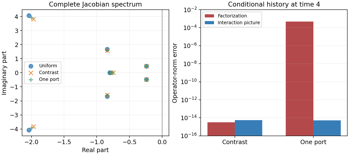
**Figure 2. Complete stability and response.** Left: all eight equilibrium Jacobian eigenvalues for each preparation, retaining multiplicities. Right: transient conditional factorization and interaction-picture errors for the two nonuniform preparations. The one-port transient relaxes to a constant carrier, but free/clamped transfer differences persist at equilibrium.
A sharp scalar curvature bound supplies an all-input sufficient attraction regime. The complete Hessian proves local stability without requiring global joint convexity. Symmetric contrast turns the stationary reduction into an exact gain law, and continuing work pays for sustained organization. Conditional phase and attenuation share a carrier; the free-memory probe retains a causal kernel. A common mean or equal power misses that distinction. The direct experiment would calibrate the energy effort, quadrature ports and memory, then compare static and phase-sensitive frequency response with and without clamping.
Time-varying drive needs a different Lyapunov argument, finite reservoirs require a supply state and depletion, and parameters outside the strict sufficient regime need separate stability analysis. Continuum limits and cross-domain microscopic identification remain open. Within the declared finite constant-input class, the construction proves attraction in its regime, quantifies gains beyond imposed preparation, and separates conditional linkage from complete response.
## References
- Jeremy Rodgers. *The Canonical Spectral-Curvature Field: A Unified Operator Origin for Coherence, Dissipation, and Spectral Budgets*. 2026a, Zenodo preprint. [DOI](https://doi.org/10.5281/zenodo.23899458).
- Jeremy Rodgers. *Adaptive Spectral Carriers: Time Ordering, Reciprocal Memory, and Linked Coherent–Dissipative Response*. 2026b, Zenodo preprint. [DOI](https://doi.org/10.5281/zenodo.23924603).
- Jeremy Rodgers. *Source Readout Non-Equivalence: Descent and Equivariant Reconstruction Obstructions*. 2026c, Zenodo preprint. [DOI](https://doi.org/10.5281/zenodo.21369967).
- Jeremy Rodgers. *Observable Quotients and Exact Projected Dynamics: Closure, Memory, Minimal Dynamical Completion, and Effective Field Operators*. 2026d, Zenodo preprint. [DOI](https://doi.org/10.5281/zenodo.21371251).
- Arjan van der Schaft and D. Jeltsema. *Port-Hamiltonian Systems Theory: An Introductory Overview*. Vol. 1 of *Foundations and Trends in Systems and Control*, nos. 2–3. Now Publishers, 2014. [DOI](https://doi.org/10.1561/2600000002).
- Robert M. Corless, Gaston H. Gonnet, D. E. G. Hare, David J. Jeffrey, and Donald E. Knuth. On the Lambert W function. *Advances in Computational Mathematics* 5:329–359, 1996. [DOI](https://doi.org/10.1007/BF02124750).
- J. P. LaSalle. *The Stability of Dynamical Systems*. Vol. 25, CBMS-NSF Regional Conference Series in Applied Mathematics. SIAM, 1976. [DOI](https://doi.org/10.1137/1.9781611970432).